Putting zero-shot learning to the test with VAEs part 3/3: A Loss function for learning disentangled latent factors

• Notice: Please see part 1 and part 2 for an introduction to this project, or if you’d like to see how I created the dataset.
• Repository for this project: Github
• Jupyter notebook used: Train_VAE_entanglement_loss.ipynb

In Brief: I first generated a synthetic image dataset by drawing from a known latent space. I train a Variational autoencoder (VAE), equipped with a modified loss function, to reconstruct input images from this dataset. This loss function includes an additional term which penalizes embeddings with high covariance among the latent variables. Its purpose is to encourage so-called “disentanglement” of latent factors, so that each latent variable might encode a qualitatively distinct high-level image feature. In this post, I’ll propose and evaluate this modified loss function, recap the VAE architecture I used, and show my results. Result: Due to the intrinsic 2-dimensionality of the dataset, the loss function may be less suitable in this case. However, the experiment illustrates how the structure of the latent embedding itself could be harnessed to identify latent factors.

Introduction

Latent factors

In the context of deep generative modeling, latent factors or generative factors can be thought of as spectra of high-level features in the set of objects comprising the dataset. These abstract spectra are called “latent” or “generative” since they effectively underlie or give rise to the objects in the dataset—each factor may represent a continuum of some particular property of the object. In the case of VAEs, these continuums are captured in the distribution of all data when it is mapped into the latent space (i.e. the ambient space of vectors output at the middle of the bottleneck). Using the example from my previous post, if a generative model such as a VAE was trained on human faces, one latent factor might encode whether or not a person is wearing glasses. As shown in the figure below, it would then be possible to identify the direction of this continuum in latent space and, using vector arithmetic, transform the latent vector corresponding to a face into the latent vector of the same face, plus glasses. Once the face+glasses latent vector is formed, you would simply use the decoder network to generate the corresponding image.

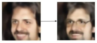
Fig. Figure Borrowed from 2

Disentanglement

One challenge deep generative modeling is to get a model to automatically learn “disentangled” latent factors. The authors of the Deepmind paper Early Visual Concept Learning with Unsupervised Deep Learning define “disentangled” as such:

We wish to learn a representation where single latent units are sensitive to changes in single generative factors, while being relatively invariant to changes in other factors.

NOTE: At this point it’s important to point out that “generative/latent factors,” in a mathematical sense, refer to directions in latent space along which high-level image features change. Whereas, “latent units” or “latent variables” will refer to the actual components of the latent vector that is output at the bottleneck of the VAE.

In other words, a disentangled set of latent factors will be such that each latent variable or latent unit encodes a qualitatively orthogonal image feature. Using the language of linear algebra/vector spaces, entangled factors occur when linear combinations of basis vectors (i.e. combinations of latent variables) are needed to define the direction of a latent factor. A disentangled representation is highly desirable for three reasons that I can see.

1. It would make combining latent variables in order to generate new images very convenient.
2. It could help automate the discovery/identification of generative factors in the dataset.
3. It could provide a path to zero-shot inference.

The authors provided this illustration and caption, which is in the same spirit as the third point.

“Models are unable to generalise to data outside of the convex hull of the training distribution (light blue line) unless they learn about the data generative factors and recombine them in novel ways”

Essentially, identifying each latent factor with a specific latent vector component could aid in generating new types of images that the model has never been trained on: zero-shot inference.

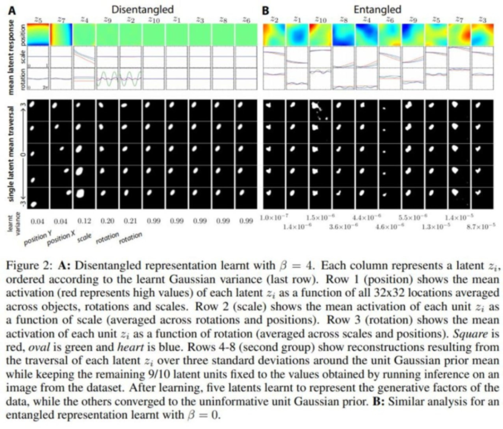
To make the concept of latent factors concrete, the Deepmind authors worked with a similar synthetic dataset consisting of images of a shape with varying x-y positions, scales, and rotations. They found that by tuning the importance of the KL loss component in the loss function, it was possible to learn disentangled latent factors. Specifically, the model encoded x-position, y-position, scale, and two types of rotation each as a separate latent unit output (borrowed Fig below). This meant that by shifting the value of one latent vector component, they could affect, for e.g., the x-position of the shape, without affecting any other of the image features.

Research Goal

The authors seemed to apply the same the loss function used in traditional VAEs. In this project, I develop and test a modified loss which is explicitly designed to encourage disentanglement of latent factors. The loss effectively penalizes both positive and negative covariance between pairs of variables in the latent space, while maintaining the original constraints imposed by the reconstruction loss and KL divergence loss.

Proposed Loss function

The rational behind my modified loss function is to apply a pressure to the latent embedding such that high positive and negative covariance between any pair of variables is costly. Theoretically, this would encourage the model to learn an embedding in which the data’s natural principle components would align with the latent variables. I.e. the data manifold should be properly oriented in the latent space so that the directions of greatest variation are parallel to the coordinate axes. This is highly connected to the linear projection that principal component analysis (PCA) performs as part of its dimensionality reduction process. PCA projects data onto a lower dimensional subspace whose basis vectors are a subset of the principal components of the original data. This means that the projected data will automatically be defined in a coordinate system aligned with the variance in the data. To achieve a similar kind of alignment of the latent embedding, we would have to precipitate it as an emergent effect of the VAE training process.

Notation

I’ll use the notation shown in the figure and table below. Note that the architecture is shown simplified. For full architecture details see the later sections below. Fig. Schematic of a basic VAE with all densely connected layers. A vector of means and log(variance) are produced as a two separate heads at the end of the encoder module. The image \(x^k\) is mapped to latent vector \(z^k\) by sampling from gaussian distributions parametrized by the means and log(variances).

Symbol	Meaning
\(z_i\)	component i of latent vector
\(x_p\)	value at pixel p of input image
\(\hat{x_p}\)	value at pixel p of output image
\(\mu_i\)	mean of component i of latent vector
\(\sigma_i^2\)	component i of variance vector
\(N\)	number of samples
\(d\)	dimensionality of latent space
\(k\)	sample index
\(w\)	image width in pixels
\(h\)	image height in pixels

In the definitions below I work with the vector of means \(\mu\) output by the dense layer at the end of the encoder. I refer to the components \(\mu_i\) as the “latent variables” rather than components \(z_i\). The \(z_i\) represent the latent vector components after gaussian noise has been added. \(z\) will then be fed to the decoder.

Deriving Entanglement loss term

You can define the covariance between a pair of latent variables as

$$Cov(\mu_i, \mu_j) = C_{i,j} = \sum_{k=1}^N \frac{(\mu_i^k - \bar{\mu_i})(\mu_j^k - \bar{\mu_j})}{N}$$

where \(C_{i,j}\) is a component of the covariance matrix. Since the KL divergence loss forces the latent embedding’s global mean along each axis towards 0 (due to the \(\mu_i^2\) term), we can assume the center of mass of the embedding will end up roughly at the origin in \(\mathbb{R^d}\). That is \(\bar{\mu_i} = 0 \forall i\). Then

$$C_{i,j} = \sum_{k=1}^N \frac{\mu_i^k \mu_j^k}{N}$$

Note: All loss functions below show the contribution to the Loss function by a single training example. In the Tensorflow code, these are in fact computed in batch, but they look similar.

One way to penalize both positive and negative covariance is to make a term that increases when these covariances increase. I will call this term the Entanglement loss:

$$L_{entg} = \frac{1}{d(d-1)/2}\sum_{i=1}^d\sum_{j=i+1}^d |\mu_i \mu_j|$$

Here we also sum over all elements in the upper triangular part of \(C\) and normalize by the number of elements in the sum. This ensures that all pairs of variables are included, and it makes the term independent of the dimensionality of the latent space. Below I plotted the loss function for 2 latent variables \(\mu_i\) and \(\mu_j\). The \(\mu_i^2\) is also included since it will be present in my final loss function.

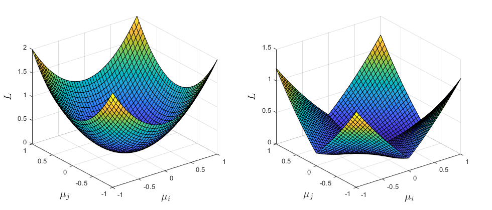Fig. (LEFT:) \(L(\mu_i, \mu_j) = \mu_i^2 + \mu_j^2\) (RIGHT:) \(L(\mu_i, \mu_j) = 0.2(\mu_i^2 + \mu_j^2) + 0.8abs(\mu_i \mu_j)\)

You can see that adding the \(L_{entg}\) term increases the loss for any points that lie on the “diagonal” directions \(y(x)=x\) and \(y(x)=-x\). This should help prevent the latent embedding from occupying these areas (or so I thought..)

Other loss components

Finally, the following losses from the normal VAE are also included in my loss:

Binary Crossentropy loss:

$$L_{crossent} = -\frac{1}{wh}\sum_{p=1}^{wh} x_p log(\hat{x_p}) + (1-x_p) log(1-\hat{x_p})$$

The average is taken over all pixels in the input and output image. Both must be normalized so that all pixels have value in [0,1].

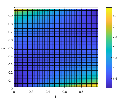
Fig. \(L_{crossent}\) as a function of the ground truth \(x_p\) and predicted \(\hat{x_p}\) values for a single pixel in the image. Yellow is higher value.

Kullback Leibler divergence loss:

$$L_{KL} = \frac{1}{2}\sum_i^d \mu_i^2 + \sigma_i^2 - 1 - log(\sigma_i^2)$$

The term \(\mu_i^2\) simply penalizes points based on how far they are from the origin. This is a major aspect of VAEs which differentiates them from vanilla autoencoders (which place no such constraint on the latent embedding). The term effectively causes latent vectors to crowd together and therefor to form a latent distribution with fewer gaps.

The second half \(\sigma_i^2 - 1 - log(\sigma_i^2)\) is a concave up function of \(\sigma_i^2\), with a minimum at \(\sigma_i^2 = 1\). It thus forces the variance towards 1.

Putting it together

Traditional VAE loss:

$$L = L_{crossent} + \beta L_{KL}$$

My Modified VAE loss:

$$L = \beta L_{KL} + L_{crossent} + \gamma L_{entg}$$

class Add_VAE_Loss(keras.layers.Layer):
    
    def compute_entanglement_loss_component(self, inputs):
        z_mean = inputs
        C_total = 0 #total 'absolute covariance' for this batch
        #cycle through each pair of latent space dimensions and compute covariance-like value. Sum over all pairs to get total covariance
        for i in range(latent_dim):
            for j in range(i+1, latent_dim):
                C_total += K.mean(K.abs(z_mean[:,i]*z_mean[:,j]), axis=0) # sum over all z_mean vectors in the batch 
        
        return C_total*2/(latent_dim*(latent_dim-1)) #we normalize by the number of elements in the upper triangular part of the cov matrix     
    
    def compute_VAE_loss(self, inputs):
        #reasonable values for coeffs: K.mean(0.001*KL_loss + 1.0*recon_loss + 0.0001*entanglement_loss, axis=0)
        sigma = 0.1
        input_image, z_mean, output_image = inputs
        KL_loss = K.mean(K.square(z_mean) + K.exp(K.log(K.square(sigma))) - K.log(K.square(sigma)) - 1, axis=1)
        entanglement_loss = self.compute_entanglement_loss_component(z_mean)
        recon_loss = keras.metrics.binary_crossentropy(K.flatten(input_image), K.flatten(output_image))
        return K.mean(0.001*KL_loss + 1.0*recon_loss + 0.0001*entanglement_loss, axis=0) #sample weight is provided as an output from the dataset (generator)
              
    def call(self, layer_inputs):
        if not isinstance(layer_inputs, list):
            ValueError('Input must be list of [encoder_input, z_mean, z_decoded]')
        loss = self.compute_VAE_loss(layer_inputs)
        self.add_loss(loss)
        return layer_inputs[2]

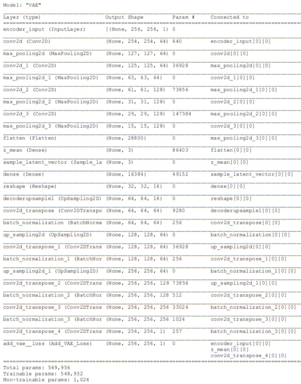
VAE architecture and training (recap)

Using the Keras-Tensorflow framework, I tested many variations on the architecture and eventually found a version which produced both excellent reconstructions and an intrinsically 2-dimensional latent vector embedding within a 3D latent space (See Figures below). The table below contains the settings I used for this experiment as well as part 2. For more details on the training and hyperparameters, see part 2. Below I’ll only cover the settings that are different from those covered part 2!

Experiment	dataset	sample weights	latent space dimensionality	Loss function	batch size	optimizer	constant variance
Parameter space transects	punctured, N=4510	yes	3	standard VAE	8	Adam	yes
Loss function for reducing latent variable covariance	full, N=5000	no	3	modified	8	Adam	yes

Fig. Tensorflow's model architecture summary.

Dataset

I used the “full” dataset containing 4499 training images and 501 validation images. This dataset did not remove 410 images that lied inside the hole region. Each image was automatically resized to 256 x 256 x 1 by the dataset generator (slightly larger dimensions than the original .png files). The training data was provided using a tf.data.Dataset, a generator object.

train_dir = 'D:/Datasets/VAE_zeroshot/data_full/processed/train' #your images must be inside a subfolder in the last folder of datadir
img_dataset_train = image_dataset_from_directory(
    train_dir, shuffle = False, image_size=(256, 256), batch_size=8, color_mode='grayscale', validation_split=None, label_mode=None)

Sample Weights

There were no sample weights used for this experiment.

Results

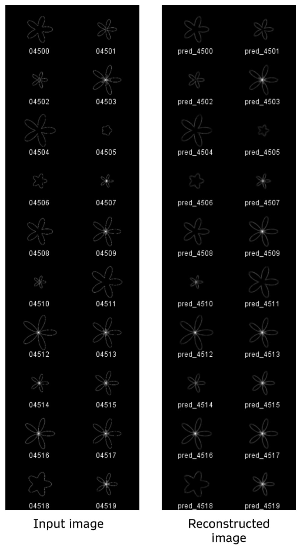
Reconstructions from validation set

Below are a sample of reconstructions made using images from the validation set as input. The validation images start at file index 4500, and I’m showing the first 20 images. The left columns are the ground truth and right columns are reconstructions of those images. The reconstructions are about the same in quality as when I used the punctured dataset in part 2.

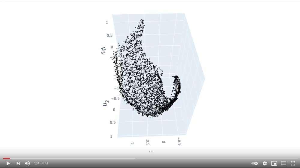
Latent space embedding

I ran multiple trainings of my model using the new loss function. For all of these, a two-dimensional data manifold emerged in the latent space. This is to be expected since the training data was composed of images drawn from a 2D parameter space (see part 1). I found that the KL divergence loss and entanglement loss were more likely to cause the edges of the embedding to curve inward than to orient the embedding along any particular axes. This is obviously not intended. However, the beauty of this experiment is the fact that we can directly observe what is happening with the embedding and the effect of the loss function on it. I believe the final orientation of the embedding after training is more sensitive to the initial conditions of the weights in the network. It was not impacted as strongly as I had hoped by the loss term.

I kept the parameters \(\beta\) and \(\gamma\) (controlling the importance of the KL and entanglement loss) small in order to preserve the 2-dimensionality of the embedding. If these parameters were increased, we would end up with a distribution closer to a multivariate gaussian, which is potentially not true to the data. The intrinsic two-dimensionality of the data suggests there are likely other datasets for which the entanglement loss is more applicable. Click to view video

Discussion | The problem with disentangled representations

How then should we go about identifying latent factors, especially in a case like this where the embedding converged upon is randomly oriented in the latent space? I propose, in future work, that we should avoid thinking of latent factors as straight lines. Implicit in the disentangled representation proposed in the Deepmind paper, is that each latent factor can be forced to correspond to a single latent unit. Changing the value of one unit while holding the others fixed should, in theory, be like turning a knob that increases the level of some property or high-level image feature.

As my results suggest, it may be difficult in many cases for a loss function alone to precipitate a disentangled latent embedding. It is possible that the latent factors are, in fact, better represented as curved lines passing through the latent space. Curved latent factors are not possible under a system where each latent factor is encoded as a single latent variable. For analogy, the gridlines of a 2D polar coordinate system curve around the origin. The direction of increasing \(\theta\) is oriented differently depending on where you are in the space. Could it be the case that a latent factor follows a curved shape within the latent embedding? For my dataset (see video) this is true. The process of vector arithmetic in the latent space would be different in this case, since you would need to follow a curved path if you wanted to increase the prominence of one image feature. In the case of my embedding, increasing the scale of the shape, for eg, would correspond to traversing a curved path that runs tangentially to the data manifold. I believe this is a manifestation of a more general property of real world datasets. It is definitely something to consider when performing generative modelling or attempting zero-shot learning.

Thanks for reading!!