Putting zero-shot learning to the test with VAEs part 2/3: Parameter Space Transects

• Notice: Please see part 1 for an introduction to this project, or if you’d like to see how I created the dataset used here. In this part, I’ll set up the ‘‘parameter space transects’’ experiment, go over the VAE architecture I used, and show my results.
• Repository for this project: Github
• Jupyter notebook used: Train_VAE_sampleweights_constant_variance.ipynb

In Brief: In the context of deep generative modeling, zero-shot learning can be thought of as a model’s ability to synthesize images that it received no training data on. I generated a synthetic image dataset by drawing from a known latent space. I removed a region of points from this dataset and trained a VAE on the remaining images. I then asked the VAE to sample images along a line extending across the removed region. Result: The model reconstructs images from the removed region fairly well in only a few cases. This highlights the difficulty of interpolating to new regions of the latent space.

Research goal | Parameter space transects

Given the ability of VAEs to interpolate between images, in this experiment I asked whether a VAE is capable of true zero-shot learning, in the sense of generating an image from a part of the latent space it has never been trained on. To make an analogy using the idea of attribute vectors, one could ask if it’s possible to generate an image of a dog wearing sunglasses, if the model saw many images of humans in sunglasses and dogs without sunglasses during training? I.e. Perhaps you could 1. find an attribute vector which is able to add sunglasses to faces, 2. add it to the latent vector corresponding to a dog photo, and 3. use the decoder network to map this dog+sunglasses latent vector back into image space.

In order to test this idea in a concrete and interpretable way, it helps to have a dataset drawn from a known, low-dimensional latent space, so that we can control exactly which parts of the space we train the VAE on. Then, we can ask the VAE to sample images directly from a part of the space it has never seen. Finally we can compare its predictions to known ground truth images from that region.

To achieve this, I generated a training set of smoothly varying images and then removed a portion of them before training. Each image is a plot of a polar function parametrized by two parameters, \((a,b)\). I will generate a “transect” across this parameter space, creating one image per point along the transect. The transect will cross directly over the removed region of the parameter space. Finally, I’ll feed these transect images to the VAE and observe their reconstructions.

Creating transect images

A “transect” in biology or any field research is a straight line along which measurements are taken. For this experiment, we are going to walk on a straight line across the 2D parameter space that the training images are generated from; this line will traverse a region of the space containing images that the VAE has never been trained on.

I construct 3 transects that cross the \((a,b)\) parameter space. \(a\) and \(b\) control the size and shape, respectively, of the polar function

$$R(\theta, a, b) = b cos(5 \theta) + a$$

plotted in training images. Each transect crosses directly over the center of the “hole” region, where points were removed from the training set.

Fig. All training images visualized in the parameter space. P1, P2, P3 are transects of 15 equally spaced points crossing the entire parameter space.

Each transect consists in 15 equally-spaced points in parameter space. In Generate_Transects.m I simply plot each polar curve along the transect and save as an image into a folder. This produces 15 images per transect that I will feed to the VAE later.

Fig. [Click to enlarge] One transect shown per row. Yellow box encloses points within the removed region.

VAE architecture and training

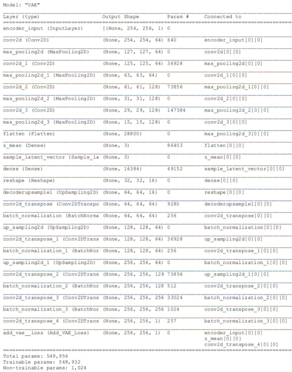
Using the Keras-Tensorflow framework, I tested many variations on the architecture and eventually found a version which produced both excellent reconstructions and an intrinsically 2-dimensional latent vector embedding within a 3D latent space (See Figures below). The table below contains the settings I used for this experiment as well as part 3. I’ll go through these in the bullet points below.

Experiment	dataset	sample weights	latent space dimensionality	Loss function	batch size	optimizer	constant variance
Parameter space transects	punctured, N=4510	yes	3	standard VAE	8	Adam	yes
Loss function for reducing latent variable covariance	full, N=5000	no	3	modified	8	Adam	yes

Fig. Tensorflow's model architecture summary.

Dataset

I used the “punctured” dataset containing 4299 training images and 211 validation images. This dataset had removed 410 images that lied inside the hole region. Each image was automatically resized to 256 x 256 x 1 by the dataset generator (slightly larger dimensions than the original .png files).

Training

I trained the model for about 30 epochs using minibatch gradient descent, with batch size 8, using the Adam optimizer with a learning rate of \(\eta = 0.0001\). The computation was performed using a NVDIA GeForce RTX2080 Ti GPU.

I stopped training approximately at the point the validation loss came close to the loss on the training data. If the training data loss drops below the validation loss, this may be a sign of overfitting. I chose not to use a testing dataset for simplicity. It reduces the amount of code. Predictions in the figures below were made using images from the validation set.

Latent space dimensionality latent_dim=3

It turned out that only 3 latent variables were needed to produce good reconstructions.

Constant Variance

One major modification, relative to standard VAEs, was to remove entirely the log-variance producing layer from the encoder. Instead, my encoder only outputs a 3D vector of means \(\mu_i\), and it samples the latent component \(z^k_i\) for image \(k\) by assuming a fixed standard deviation of \(\sigma_i = 0.1\) for all variables \(z_i\). This causes the probability distribution of the latent vectors to be spherical and identical in size for all images. Since the log-variance layer is a dense layer, the total number of parameters in the network also drops substantially after removing it. I found that allowing the model to skip learning how to output log-variances actually sped up training and improved performance. However, the reason for this may have had to do with using an improper activation function on my log-variance layer.

z_mean = layers.Dense(latent_dim, activation='linear', name='z_mean', kernel_initializer='RandomNormal',  bias_initializer='zeros')(x)

class Sample_latent_vector(keras.layers.Layer):
    def sample(self, inputs):
        sigma = 0.1
        z_mean = inputs
        epsilon = K.random_normal(shape=K.shape(z_mean))
        return z_mean + epsilon*sigma
    
    def call(self, inputs):
        return self.sample(inputs)
    
z = Sample_latent_vector()(z_mean)

Linear activation on \(\mu\)

On the layer z_mean producing latent component means \(\mu_i\), I found that a linear activation was best for ensuring that the encoder mapped the training set to a 2-dimensional, sheet-like, embedding (within the 3D latent space) See figures.

Sample Weights

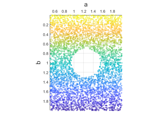
I tried applying sample weights so that my “starfish” shapes with shallower waves (lower \(b\)) were weighted more heavily in the loss function. This had little effect on the quality of the reconstruction. However sample weights might have greater with other datasets. The quality was more strongly impacted by other factors such as using different activation functions on the log-variance layer (before it was removed). The figure below colorizes the weight used for each sample. I used a scheme in which weights were directly proportional to \(b\) and occupied the range \([0,1]\).

Note: I couldn’t get Tensorflow’s built-in sample weight generator to work, so I had to provide sample_weights as a separate input to the model. This was done by constructing a customized tf.data.Dataset object which can generate input data as tuples. These tuples contain batches of images, their corresponding weights, and intended output images.

Fig. Weighted Training dataset visualized in parameter space. Color indicates the values sample_weights applied to each sample in the loss function. Yellow is higher value, purple is low. This weighting scheme causes the loss function to increased by more when errors are made on samples with shallower waves (lower b)

Standard VAE loss (almost)

The loss function used is the standard VAE loss: a combination of an image reconstruction loss and a Kullback Leibler divergence loss. In part 3 I will recap this loss function and test out a novel loss function. Notice that since I’m working with a constant variance of \(\sigma_i^2 = 0.1^2\), I can simply substitute this constant into the loss function (as opposed to providing an entire log-variance tensor).

class Add_VAE_Loss(keras.layers.Layer):
    
    def compute_VAE_loss(self, inputs):
        sigma = 0.1
        input_image, z_mean, output_image, sample_weights = inputs
        KL_loss = K.mean(K.square(z_mean) + K.exp(K.log(K.square(sigma))) - K.log(K.square(sigma)) - 1, axis=1)
        recon_loss = keras.metrics.binary_crossentropy(K.flatten(input_image), K.flatten(output_image))
        return K.mean((8e-3 * KL_loss + 1*recon_loss)*sample_weights*2, axis=1) #sample weight is provided as an output from the dataset (generator)
        
        
    def call(self, layer_inputs):
        if not isinstance(layer_inputs, list):
            ValueError('Input must be list of [input_image, z_mean, output_image]')
        loss = self.compute_VAE_loss(layer_inputs)
        self.add_loss(loss)
        return layer_inputs[2]

Results

Reconstructions from validation set

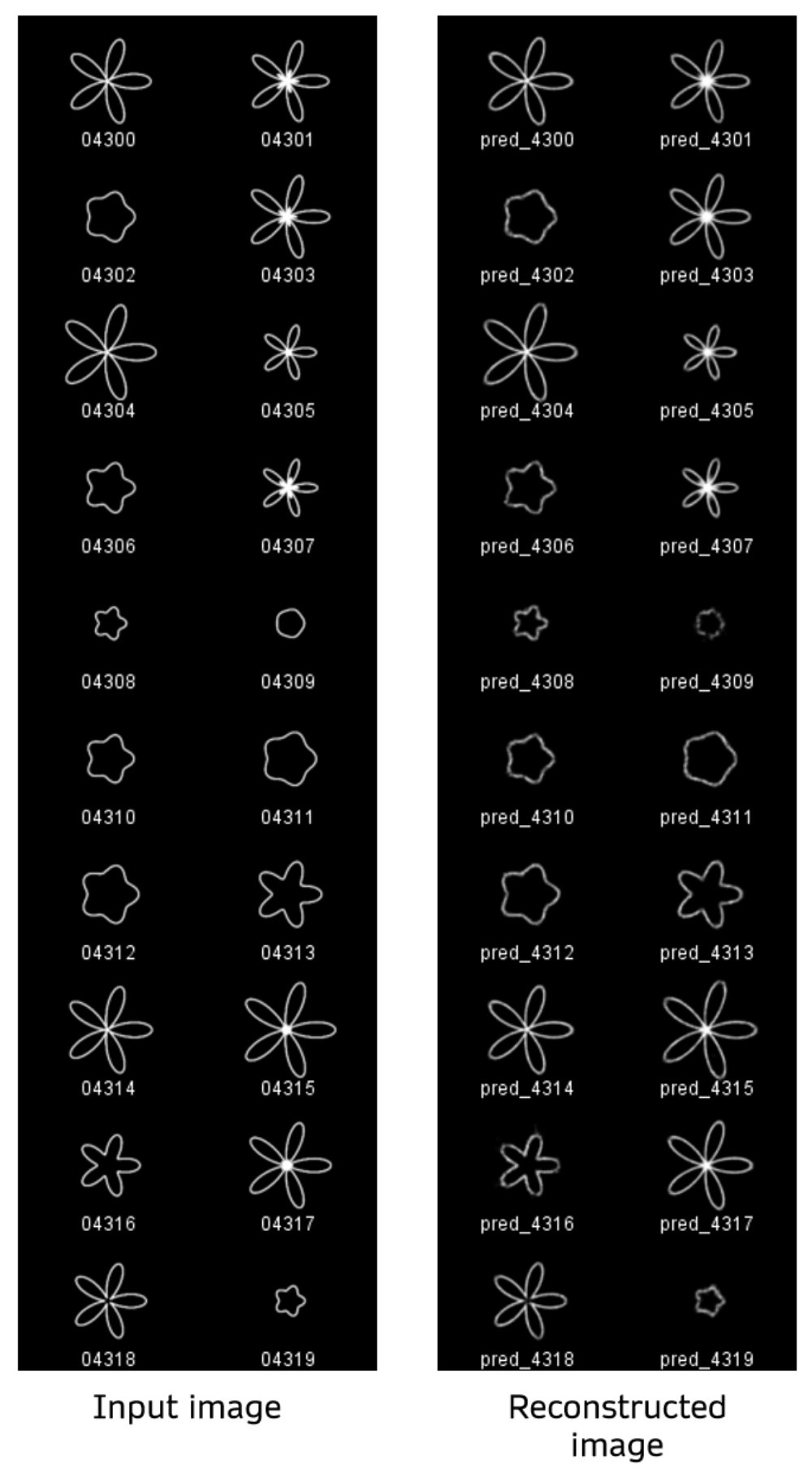
Below are a sample of reconstructions made using images from the validation set as input. The validation images start at file index 4300, and I’m showing the first 20 images. The left columns are the ground truth and right columns are reconstructions of those images. Among all versions of the model I prototyped, including the one used here (see Train_VAE_sampleweights_constant_variance.ipynb), shapes with shallower petals and smaller sizes were the most difficult to reconstruct well. I did not quantify the reconstruction loss on these images but just estimated by eye. This motivated my experiments where I applied higher sample weights to certain images. The sample weights did not have a profound effect in this case, relative to changing other architectural features such as activation functions and batch norm layers in the encoder. Still, the difficulty in reconstructing certain shapes probably stems from imbalances in the dataset itself. The smaller and low-curvature shapes are effectively under-represented in the data since the larger and high-curvature shapes are more similar to each other. The majority of convolutional filters learned likely respond to image features present in the high-curvature shapes. There was possibly less priority to learn filters that respond to the low-curvature features due to their scarcity in the dataset.

Latent space embedding

In order to obtain latent vectors, I created a version of the encoder which is identical except that the sampling layer sample_latent_vector is removed. As such, the latent vectors shown in these results are taken to be the vectors of latent component means \(\mu\). To do this you copy layers from the original model to a new model. The learned weights of the layers in the new encoder can either be loaded in before or after creating it. I chose to load the weights in first and then copy the layers to a new model as below

VAE = keras.models.load_model(r"C:\Users\MrLin\Documents\Experiments\VAE_zeroshot\VAE_weighted_const_variance")
detached_encoder_input = Input(shape=(256, 256, 1), name='detached_encoder_input')
x = detached_encoder_input #
for layer in VAE.layers[1:15]:#we must skip the VAE input layer (for loop starts at layer 1 instead of 0) as it causes problems to use the same input layer in two separate models
    x = layer(x)
    
encoder = Model(detached_encoder_input, x, name='encoder')

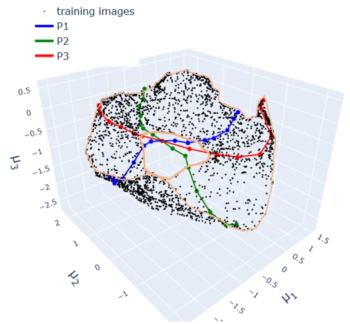
When viewed in the 3D latent space, the set of all training images forms a intrinsically 2-dimensional (sheet-like) data manifold (See YouTube video). This is unsurprising considering that

1. The images are drawn from a 2D parameter space
2. They are sampled densely enough to cover the entire space of possibilities (besides in the hole region)
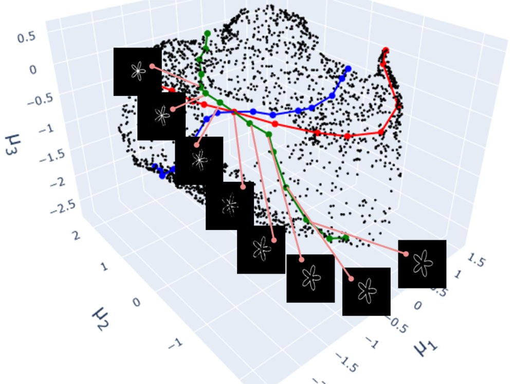
3. The images change continuously: small changes in the parameters lead to small changes in the corresponding images. This means too that any image \(x^k\) can be smoothly deformed into another \(x^l\) by “walking” across the dataset in the direction of the desired destination image. This is essentially what each transect of images, denoted by P, does.

Fig. Latent space embedding with transects. Several transect images on P2 are connected by a pink line to their corresponding latent vector.

Fig. Latent space embedding with transects. I added a beige line to illustrate the boundary around the hole region and outer edge of the sheet.

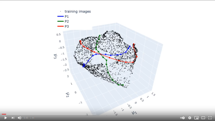Click to view video

Transect reconstructions

Finally, I used the VAE to reconstruct all transect images. I did not quantify the reconstruction error but it is evidently lower on points inside the hole region. The conditions for learning in this experiment were designed to give the model the best chance of achieving zero-shot learning. The “hole” region of the latent space we trying to sample from had many training samples surrounding it. It is perhaps surprising that model still struggled to make inferences on this unseen region in several cases. The reconstruction errors in the hole highlights the difficulty of extrapolation that is, in principle, required for real zero-shot learning in generative models.

In part 3, I’ll run a different experiment that helps expose the underlying causes of this issue.

Fig. Transect reconstructions. [Click to enlarge] The top row of each pair of rows shows the ground truth and the bottom rows show the VAEs reconstructions. The yellow box encloses points from within the hole region.