In Brief
- In the context of deep generative modeling, zero-shot learning can be thought of as a model’s ability to synthesize images that it received no training data on. This can, in theory, be achieved by combining latent variables in new ways.
- I perform two experiments in that involve training generative models called Convolutional variational autoencoders (VAE) on a synthetic image dataset, drawn from a known, 2D latent space.
- By engineering the latent space directly, I evaluate the VAE’s ability to perform zero-shot learning in a highly interpretable experiment.
-
Experiment 1, Parameter space transects (part 2/3) I first remove a region of points from the center of a synthetic image dataset. Then I use the trained VAE to sample images from the removed region. Result: The model reconstructs images from the removed region fairly well in only a few cases. Highlights the difficulty of interpolating to new regions of the latent space. -
Experiment 2, A Loss function for reducing covariance between latent variables (part 3/3) I train the same VAE on the full image dataset. Here I develop and test a modified loss function designed to minimize covariance between variables in the latent space. The purpose of this loss function is to encourage “disentanglement” of the latent variables, such that each variable encodes a qualitatively orthogonal spectrum of image features. Result: The intrinsic two-dimensionality of the training data was confirmed by examining its distribution in a 3D latent space (output of the encoder network). The loss function did not force disentanglement of the latent variables. - In this post (part 1/3): I show how we construct the image dataset with a known latent space.
Introduction
Within deep learning, deep generative modeling deals with models that can generate new images, sound, text, or other rich forms data that would typically be used as the inputs to deep neural nets. Some of the most famous examples in computer vision include generation of never-before-seen human faces using GANs, “deep dream” images, and the transfer of the artistic style of a painting to a photo (style transfer). In this 3-part series I’m going to focus on a type of generative model called variational autoencoders (VAE). I’ll cover experiments where we test VAEs’ abilities to perform “zero-shot learning,” explained later. An in-depth explanation of VAEs is beyond the scope of this post but I’ll mention some of the key points. Check out these sources which give great intros on VAEs: Variational autoencoders, Intuitively Understanding Variational Autoencoders, Understanding VAEs, Generating new faces with Variational Autoencoders.
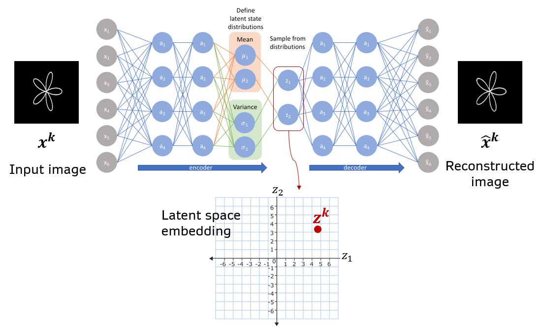 Fig. Schematic of a basic VAE with all densely connected layers. A vector of means and log(variance) are produced as a two separate heads at the end of the encoder module. The image \(x^k\) is mapped to latent vector \(z^k\) by sampling from gaussian distributions parametrized by the means and log(variances).
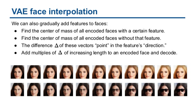
VAEs have some key advantages that make both their training and interpretation easier than in more complex models such as GANs. Like vanilla autoencoders, VAEs can train in a totally unsupervised regime, where the network is tasked with taking in an input image and reconstructing it as output. The data’s ground truth labels are the inputs. VAEs are also capable, by design, of learning a continuous latent space, from which new samples (images) can be drawn. The latent space refers to the set of underlying variables that control high-level features in the set of objects comprising the dataset. In mapping human faces to a latent space, for example, perhaps there are axes which directly affect masculinity/femininity of the face. In terms of VAE architecture, the latent vector \(\mathbf{z}\) refers to the vector at the middle of the bottleneck (see fig). In contrast to autoencoders, VAEs sample this vector probabalistically by drawing each vector element \(z_i\) from a normal distribution with mean \(\mu_i\) and standard deviation \(\sigma_i\). We can thus think of an image as being mapped to a probability distribution in latent space. And the shape of this distribution is a multivariate gaussian (ellipsoid-like). \(\mu_i\) and \(\sigma_i\) are themselves output by two separate ‘heads’ of the encoder network. By effectively adding noise to the location of the latent vector, we encourage the VAE to produce a smooth latent space, where small changes in the latent vector lead to small changes in the image generated by the decoder. In addition to the image reconstruction loss, VAE’s also include a Kullback Leibler divergence loss which forces latent vectors to cluster near the origin. This force helps prevent gaps in the distribution of latent vectors and therefore allows better interpolation between two images (see Variational autoencoders). In addition to allowing smooth interpolation between images, the latent space learned by VAEs has even been shown to support “attribute vectors” and arithmetic using such vectors (see Latent Variable Modeling for Generative Concept Representations and Deep Generative Models).
Research goal | Experiment 1, Parameter space transects
Given the ability of VAEs to interpolate between images, in this experiment I asked whether a VAE is capable of true zero-shot learning, in the sense of generating an image from a part of the latent space it has never been trained on. To make an analogy using the idea of attribute vectors, one could ask if it’s possible to generate an image of a dog wearing sunglasses, if the model saw many images of humans in sunglasses and dogs without sunglasses during training? I.e. Perhaps you could 1. find an attribute vector which is able to add sunglasses to faces, 2. add it to the latent vector corresponding to a dog photo, and 3. use the decoder network to map this dog+sunglasses latent vector back into image space.
In order to test this idea in a concrete and interpretable way, it helps to have a dataset drawn from a known, low-dimensional latent space, so that we can control exactly which parts of the space we train the VAE on. Then, we can ask the VAE to sample images directly from a part of the space it has never seen. Finally we can compare its predictions to known ground truth images from that region.
To achieve this, I generated a training set of smoothly varying images and then removed a portion of them before training. Each image is a plot of a polar function parametrized by two parameters, \((a,b)\). In part 2 I will generate a “transect” across this parameter space, creating one image per point along the transect. The transect will cross directly over the removed region of the parameter space. Finally, I’ll feed these transect images to the VAE and observe their reconstructions.
Generating the dataset
I wrote matlab code Generate_latent_space.m that can be found in this repository to generate and save the images. Each image plots a polar function defined by
where \(\theta \in [-\pi, \pi]\) and \((a,b)\) are fixed and define the point in the parameter space that corresponds to one image. \(a \in [0.5, 2]\) controls the radius of the circle and \(b \in [0, 2]\) controls the amplitude of oscillations superimposed on the circle. In the figure below I varied \((a,b)\) over a 10x10 grid in parameter space.
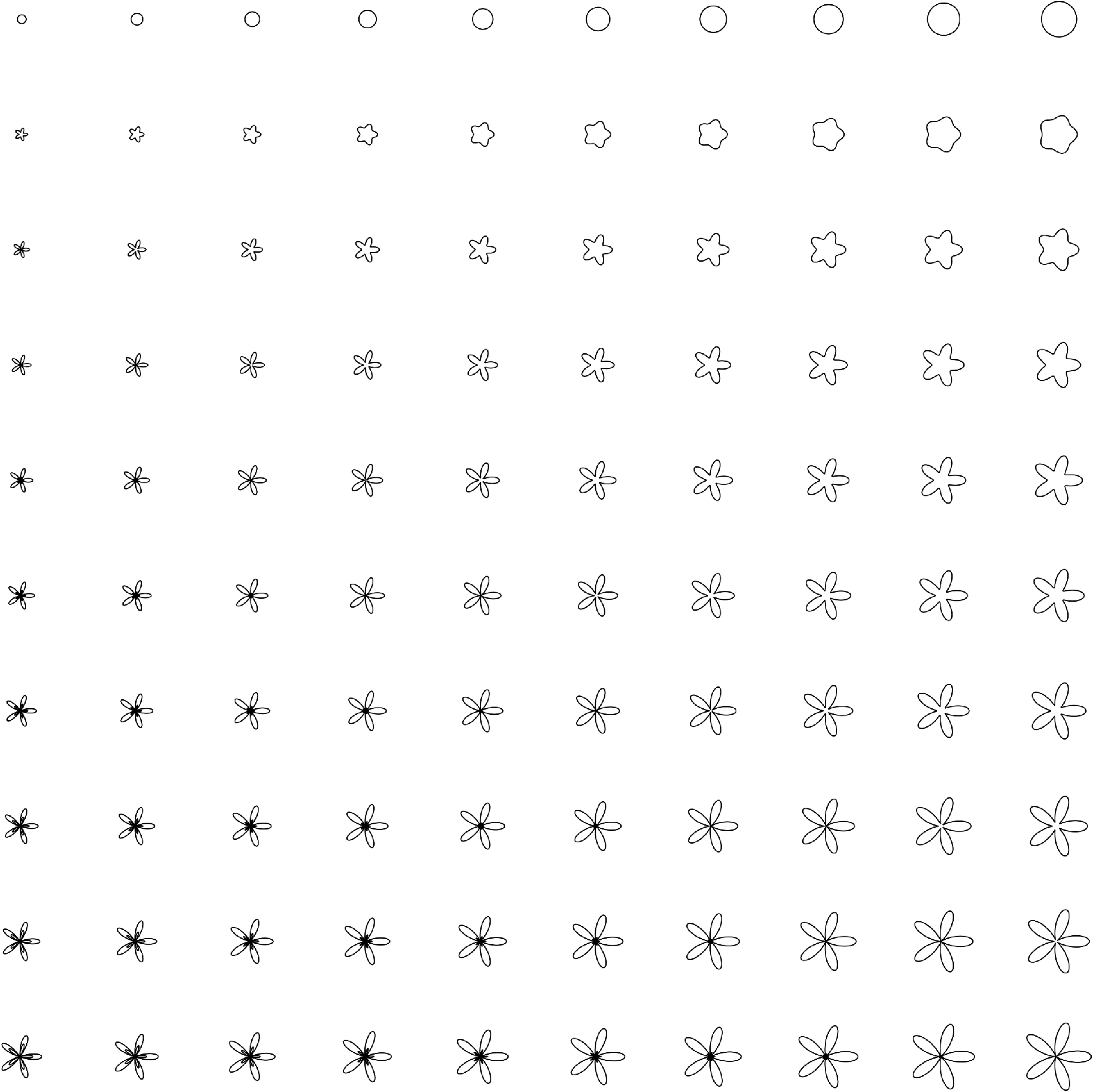 Fig. Grid sampling of images over a 10x10 lattice in the parameter space. The x-axis corresponds to varying \(a\) and the y-axis corresponds to \(b\).
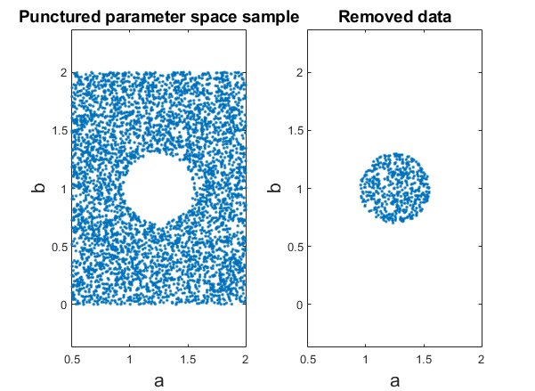
To generate the full dataset I sampled 5000 points uniformly at random over the range of the parameter space. I then chose a circular region of radius \(r=0.3\) centered at \((a=1.25, b=1)\), and I removed all points inside the region from the dataset.
Npoints = 5000;
data_full = [1.5*rand(Npoints,1)+0.5, 2*rand(Npoints,1)]% [a b]

puncture_location = [1.25 1];
puncture_radius = 0.3;

dists = pdist2(data_full, puncture_location);
data_punctured = data_full(dists>puncture_radius,:);
Finally I plot each curve and save it to the training set folder. The latter 500 of the 5000 images were moved to a testing dataset folder later. I did some additional image processing steps using Fiji/Imagej, such as inverting the images, that are not important. The .mat file containing the matlab workspace is also included in my repository if you’re interested.
R2 = @(th, a, b) b*cos(5*theta) + a;
m=4;
for j = 1:length(data_punctured)

    [x,y]=pol2cart(theta, R2(theta, data_punctured(j,1), data_punctured(j,2)));
    h=plot(x,y,'k','linewidth', 2)
    axis([-m m -m m])
    axis equal
    axis off
    h=gcf
    saveas(h, ['D:\Datasets\VAE_zeroshot\data_punctured_1p25-1_R0p3\img_' sprintf('%04d',j) '.png'])
    close(h)

end
Sample of training images
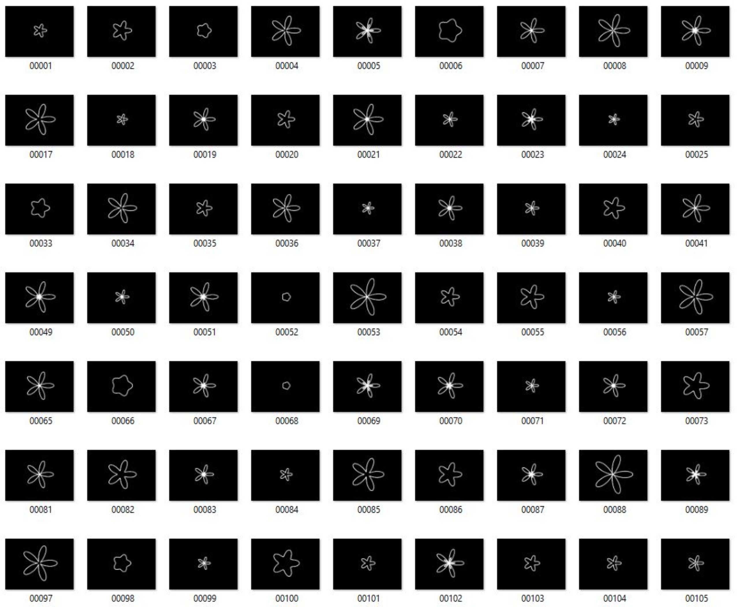 Fig. Sample of processed training images