
Parallelized Algorithms for computing large Similarity Matricies
Fast-similarity-matrix repository
In this post I’m going to demonstrate three algorithms for computing large symmetric similarity matrices (in this case, 20000 x 20000). The first is a baseline approach that we will use as a benchmark to measure the performance of the latter two. Algorithm 1 and 2 compute the matrix by distributing the work across multiple parallel workers. Algorithm 1 achieves a 6x speed up. Algorithm 2 achieves a 14.3x speed up but is more memory-intensive than algorithm 1. I use python’s concurrent.futures, concurrent.futures.ProcessPoolExecutor(),
and the computation was performed on a Ryzen 9, 12 core, 24 thread processor, 3.8GHz base.
| Algorithm | Description | Time elapsed (s) | relative speed | speed up |
|---|---|---|---|---|
| 0 | loop through each pair | 1376 | 1 | 0 |
| 1 | send inner loop to workers | 229 | 0.1664 | 6.00 |
| 2 | sum component-wise distance matricies | 96 | 0.0698 | 14.33 |
Parameters used for all algorithms
I will be computing the similarity matrix using a synthetic dataset of 20000 uniformily distributed points in 4-dimensional space.
N = 20000 #number of data points
D = 4 #dimensionality of data
tau = 0.05 #optional similarity cutoff
dat=np.random.rand(N,D)
The tau will be used for creating sparsity in the matrix so that it can be stored in sparse matrix format. This is optional but will reduce the memory used to store the matrix.
Baseline algorithm: cycle through all pairs of data points
See Fast_similarity_matrix.ipynb
In this naive approach, we simply loop through all elements in the lower triangular part of the matrix and record the distance separating each pair of points. This assumes the matrix should be symmetric, which is the case for most types of similiarity matrices. It also assumes the elements on the diagonal are not needed.
W = np.zeros((N,N), dtype=float) #similarity matrix to be filled in
#fill lower triangular part only
for i in np.arange(1,N):
    for j in np.arange(i):
        W[i,j] = F.dist(dat[i,:],dat[j,:])
We then apply the gaussian similarity function and threshold the resulting similarity values by tau, effectively setting the most distant points to have zero similarity. This obviously discards some information on the global structure of the data. The effect of doing this is the subject of another post! The benefit of creating sparsity is that we can reduce the amount of memory used to store the matrix. Here I use the scipy COOrdiate sparse matrix format.
sigm = lambda x : np.exp(-x**2/(2*0.3**2)) #gaussian similarity function or kernel
Q = sigm(W)
Q[Q==1]=0 #set upper triangle to 0 (it should hold 1's currently)

#threshold to increase sparsity, sacrificing some information
Qthresh = Q.copy()
Qthresh[Qthresh<=tau] = 0
#convert to COOrdinate format sparse matrix
Qthresh_coo = coo_matrix(Qthresh)
Memory use
| Matrix | description | size (.nbytes) (GB) | size (sys.getsizeof) (bytes) |
|---|---|---|---|
| Q | dense similarity matrix | 3.2 | 3.2E+09 |
| Q_coo | sparse version of Q, coo format | 3.19984 | 48 |
| Qthresh | thresholded dense matrix | 3.2 | 3.2E+09 |
| Qthresh_coo | sparse version of Qthresh | 1.37335 | 48 |
Algorithm 1: Each processor computes the distances for a single data point
In this method we allow each CPU worker to compute the distances for a different data point. That is, the inner loop of the baseline algorithm is delegated to one worker so that the rows of the matrix are computed in parallel. This algorithm calls the method row_similarity in Fast_similarity_matrix_func.py. The function and the data needed by each CPU worker is distributed using concurrent.futures.ProcessPoolExecutor().
To do this we must create lists of each parameter and a corresponding list of copies of the data set: [dat for _ in range(N)].
ROW = list(np.arange(1,N))
TAU = [tau for _ in range(N)]
Each worker will receive one element of these lists at the same index. There may be a way to avoid creating a list of copies of the dataset, but I haven’t gone that far with this method. ROW contains the list of row indices; each worker will receive one row to process and will use the row_similarity method shown later.
data=[]
rows=[]
cols=[]

with concurrent.futures.ProcessPoolExecutor() as executor:
    results_generator = executor.map(F.row_similarity, [dat for _ in range(N)], ROW, TAU) #

#append each peice of data sent back from the workers to a list of arrays
    for i in results_generator:
        if i[0]: #if nonempty
            data.append(np.array(i[0]))
            rows.append(np.array(i[1]))
            cols.append(np.array(i[2]))

# print(data)
    data = np.concatenate(data, axis = 0)
    rows = np.concatenate(rows, axis = 0)
    cols = np.concatenate(cols, axis = 0)
    Q_PPEmap = coo_matrix((data, (rows, cols)), shape=(N,N))
The data,rows, and cols (used by the scipy coo format) seem to be returned in the order they are completed. We can simply append all incoming data returned by row_similarity together and later convert it to coo matrix format. Below are the functions given to each worker.
def dist(x, y):
    return np.sqrt(np.sum((x-y)**2))

def sigm(d):
    return np.exp(-d**2/(2*0.3**2))

def row_similarity(dat, row, tau):
    #dat: data matrix
    #row: what row index this worker is in charge of looping across
    #tau: similarity threshold
    row_arr = []
    col_arr = []
    data = []
    for j in np.arange(row):
        if sigm(dist(dat[row, :], dat[j, :])) >= tau:
            data.append(sigm(dist(dat[row, :], dat[j, :])))
            row_arr.append(row)
            col_arr.append(j)
    return data, row_arr, col_arr
Note that the value of tau may affect the speed of this since we do not append similarity values below tau. A totally fair comparison with the baseline algorithm would use tau = 0, but the majority of the speed up should be due to the parallelization and not to skipping some pairs of points.
Algorithm 2: Component-wise computation
In this method we split the computation into \(D\) components, where \(D\) is the dimensionality of the data. Each worker receives one dimemsion and computes a distance matrix on that dimension only. These component-wise distance matrices are ultimately added together to obtain the full distance matrix. The method is much more memory intensive since each CPU processor must do matrix operations on large matricies. The speed up in this case comes from using vectorized operations.
Let \(O\) be the data matrix where rows are \(N\) observations in \(D\) dimensions. We will tile the \(j^{th}\) column of \(O\) horizonally to form matricies \(C\) and \(C^T\)
\(j^{th}\) column of \(O\):
\[x_j = [O_{1,j}, O_{2,j}, ...,O_{N,j}]^T\]\(C_j\) (a tiling of \(N\) repetitions):
\[C_j = [x_j, x_j, ..., x_j]\]The distance matrix can then be computed as
\[W = \sqrt{\sum_{j=1}^D (C_j - C_j^T)^2}\]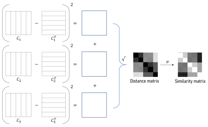
We again use the concurrent.futures.ProcessPoolExecutor(). However, this method will not utilize all processors unless the dimensionality of the data exceeds the processor count. Run multiprocessing.cpu_count() to check. This time we call the componentwise_similarity method.
Nlist = [N for _ in range(D)]
Dlist = [d for d in range(D)]
M = np.zeros((N,N), dtype=float)
with concurrent.futures.ProcessPoolExecutor() as executor:
    result_generator = executor.map(F.componentwise_similarity, [dat for _ in range(D)], Dlist, Nlist)
    for d in result_generator:
        M += d

    sigm = lambda x : np.exp(-x**2/(2*0.3**2))
    M = sigm(np.sqrt(M))
    M[M<tau]=0
    M[M==1]=0
    QM = coo_matrix(np.tril(M))
From the module Fast_similarity_matrix_func.py handed to each worker:
def componentwise_similarity(dat, dim, N):
    #dim: dimension of input vectors to take the difference in
    #dat: data matrix
    col_tile = np.tile(np.expand_dims(dat[:, dim], axis=1), (1, N))
    row_tile = np.transpose(col_tile)
    return (col_tile - row_tile)**2