t-SNE Implementations with more flexible similarity metrics in the embedding space

A more flexible similarity metric than the students-t distribution

My “t-SNE” repository includes matlab functions which implement customized versions of t-SNE. The main difference from the original paper is the use of a different similarity metric in the embedding space. This function allows you to more intuitively tune and explore the embedded result.

For all scripts I use a modified similarity function (as opposed to the student’s t distribution) for computing the similarity of two points in the lower dimensional embedding. This function can be tuned more intuitively using the bulge and fan parameters. If d is the distance between two points, their similarity is computed as

(1+d.^bulge).^-fan

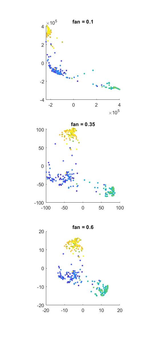
The fan parameter allows additional tuning of cluster density

Tuning these parameters can produce dramatically different results. By decreasing fan one can increase the thickness of the function’s tails. Thicker tails will grant more similarity to pairs of points which are futher apart. With thicker tails (lower fan), the large scale structure appears to become more flexible, and the algorithm will form denser clusters (similarly to decreasing the perplexity perp, see below). In contrast, with higher fan, you tend to get less dense clusters and the global geometry of the data manifold seems better preserved.

Original 3D data consists of 3 clusters. Color indicates cluster membership.

Fig. Higher `fan` causes thinner tails of the similarity function in the embedding space and less dense clusters.

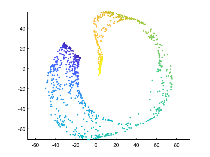
Swiss roll dataset

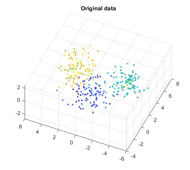
For all comparisons below I use the 3D “swiss roll” dataset and reduce it into 2D. As t-SNE is an iterative process, I also use the exact same initial condition: points are drawn from a bivariate normal distribution in 2D.

tSNE_simple.m

This modified t-SNE skips the computation of neighborhood sizes σ, and instead uses the same neighborhood size for each point. This is equivalent to computing a similarity matrix using a radial basis function/kernel and a euclidean distance metric.

tSNE_perplexity.m

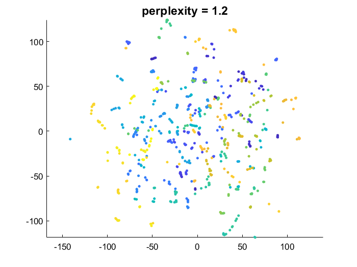
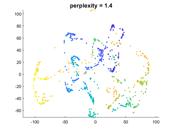
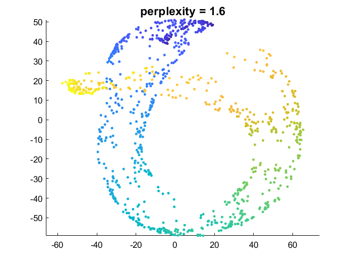
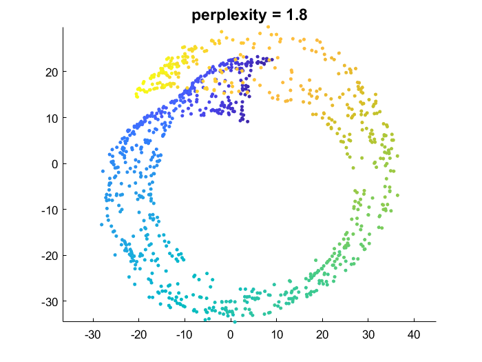
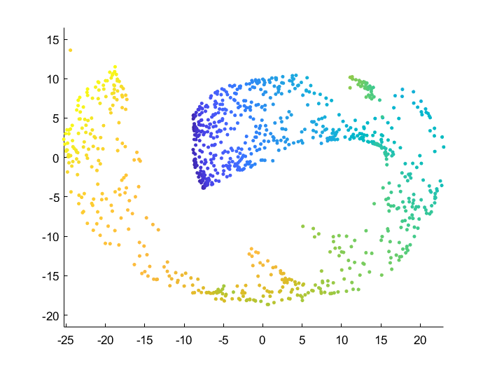
This implementation is very close to the original paper [1]. A unique neighborhood size is optimized for each point. The function takes the perplexity perp as an argument. You can also specify the initial condition Y0 and the bulge and fan parameters. The lower the perplexity, the greater the emphasis on preserving local/small scale data structure, and the more flexibility on global data structure. Higher perplexity makes t-SNE try to better preserve global data manifold geometry (making the result closer to what PCA would do).

• low perplexity: points which are close in the high dimensional space are forced to be close in the embedding. But points that are far apart are allowed to be either close or far in embedding
• high perplexity: points which are close in the high dimensional space are forced to be close in the embedding. But for points that are far apart t-SNE tries harder to make them far in the embedding. The nature of dimensionality reduction means it’s NOT always going to be possible to guarantee this second condition (overlap is common).

tSNE_Prefab_similarityMatrix.m

This function allows you to perform a t-SNE like dimensionality reduction, but skipping the computation of similarities in the original high-dimensional space. Instead you can provide a prefabricated similarity matrix P and the algorithm will pick up from that point as normal.

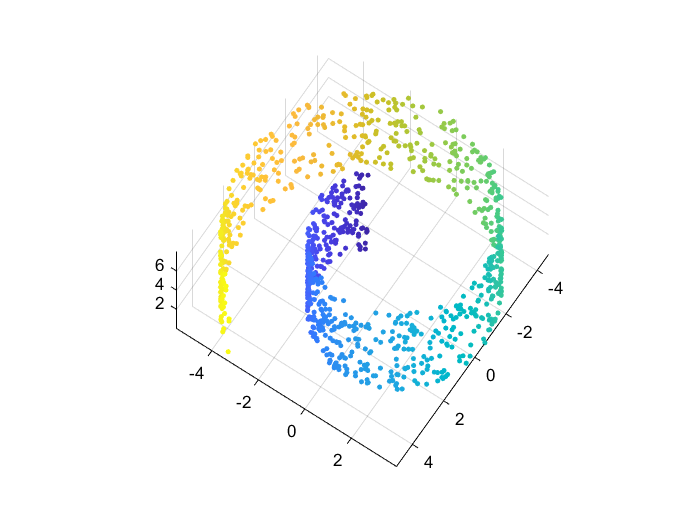
Here I computed a similarity matrix from the raw swiss roll data and then fed that to tSNE_Prefab_similarityMatrix.m

dat=load('swissroll'); dat=dat.dat; 
P=squareform(pdist(dat,'euclidean'));
G=@(d,sig) exp(-d.^2/(2*sig^2));
W=G(P,1.5);
emb=tSNE_Prefab_similarityMatrix(W,2,100);

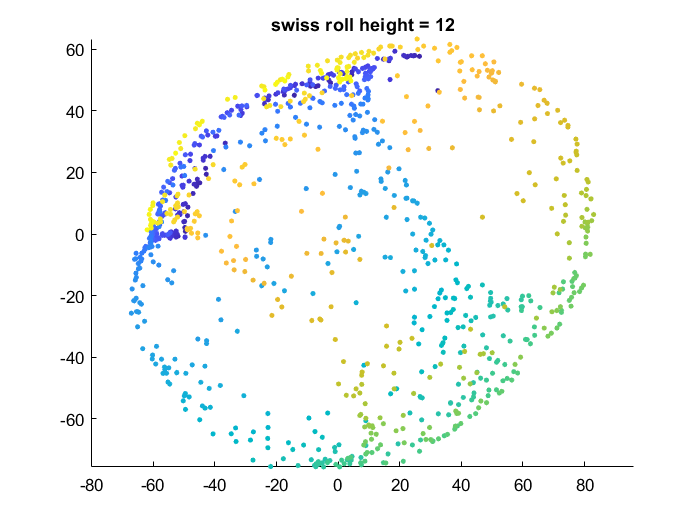
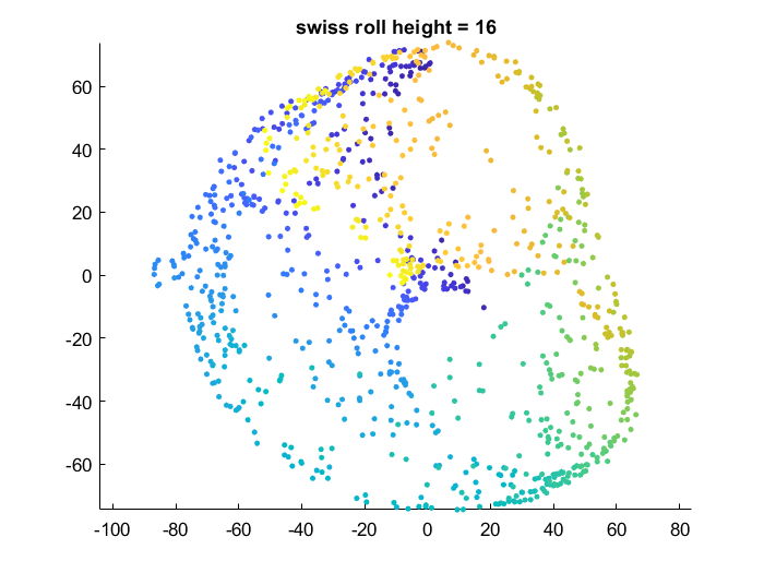
Effect of data manifold shape

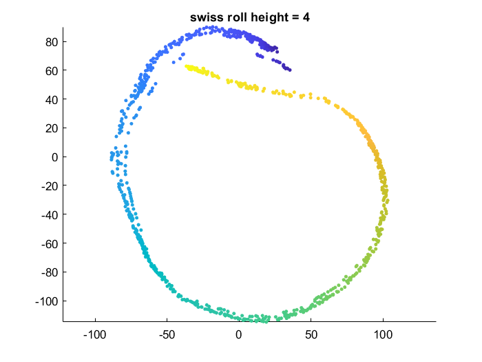
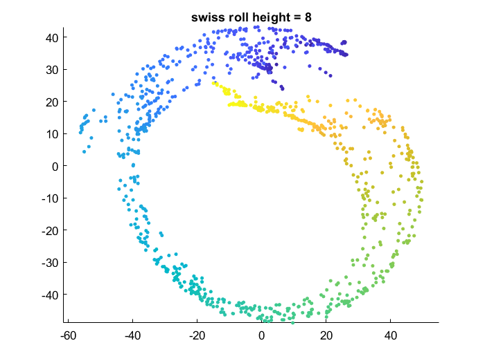
Below I vary the height of the swiss roll given to t-SNE (length of data along z axis), and fix the perplexity at 1.7. There is a transition as embedding captures more of the variation along the z-axis. At the same time, the embedding begins to not physically separate points at different lengths along the roll, creating false overlap.

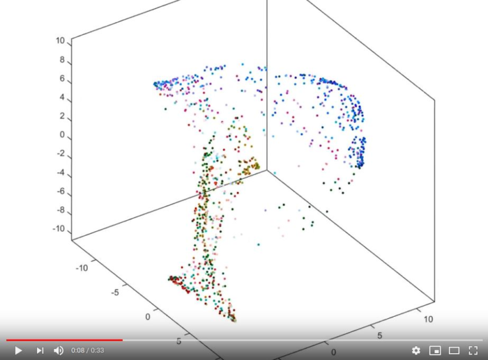
Visualization of how points are rearranged over time

This clip shows how initially randomly distributed points are moved by the algorithm over time steps. This video is for a different data set but the process would be similar for the swiss roll.

References

1. Maaten, Laurens van der, and Geoffrey Hinton. “Visualizing data using t-SNE.” Journal of machine learning research 9.Nov (2008): 2579-2605.