- part 1: An introduction to this project and links to the github repository.
- part 2: A list of subtasks involved with this project.
- part 3: The experimental setup, dataset, and definition of input tensors and targets.
Understanding the ConvLSTM layer
Making sense of what exactly the convolutional LSTM is doing is probably the biggest hurdle to overcome for those trying to understand why this model works well for this dataset and problem. For one thing, the dimensionality of the model has been increased by one, relative to 2D CNNs. The input is now a 4D tensor (time-steps, height, width, channels)! Include the batch axis and now you have 5 dimensions: (samples, time-steps, height, width, channels). To most people, I’d imagine that makes things quite a bit harder to visualize..
One can always gain a high-level understanding, of any model, by just viewing it as a black box function that takes in some input, performs some computations, and produces some output. (In part 1 I gave a broad overview of the ConvLSTM and how it has been applied in video synthesis or video prediction problems. Take a look at the papers referenced there.) To get a deeper understanding of the ConvLSTM, its helpful to compare it with traditional LSTMs. Unfortunately, it’s outside the scope of this article to go into detail on this. However, I’ve drawn up a 3D model of all the tensors and convolution kernels involved in a ConvLSTM. To my knowledge, no one in the literature has attempted to visualize the mechanics of the model to this level of detail.
I’ve drawn this schematic based on the vanilla ConvLSTM equations initially presented in the seminal work Convolutional LSTM Network: A Machine Learning Approach for Precipitation Nowcasting (2015). These are shown below, but please see the paper for details. If you are familiar with the standard LSTM equations, you’ll notice many parallels in how the gates are computed. In the case of ConvLSTM, the inputs, hidden states, memory cells, and gates are all 3D tensors. The weights \(W\), shown in the top two rows of my schematic ConvLSTM_Cell, are presented as single symbols in the equations, but in actuality they represent a bank of convolution kernels. This was very confusing to me initially.
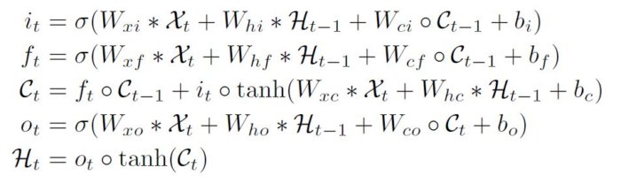 Fig. Unmodified ConvLSTM equations Shi et al. 2015
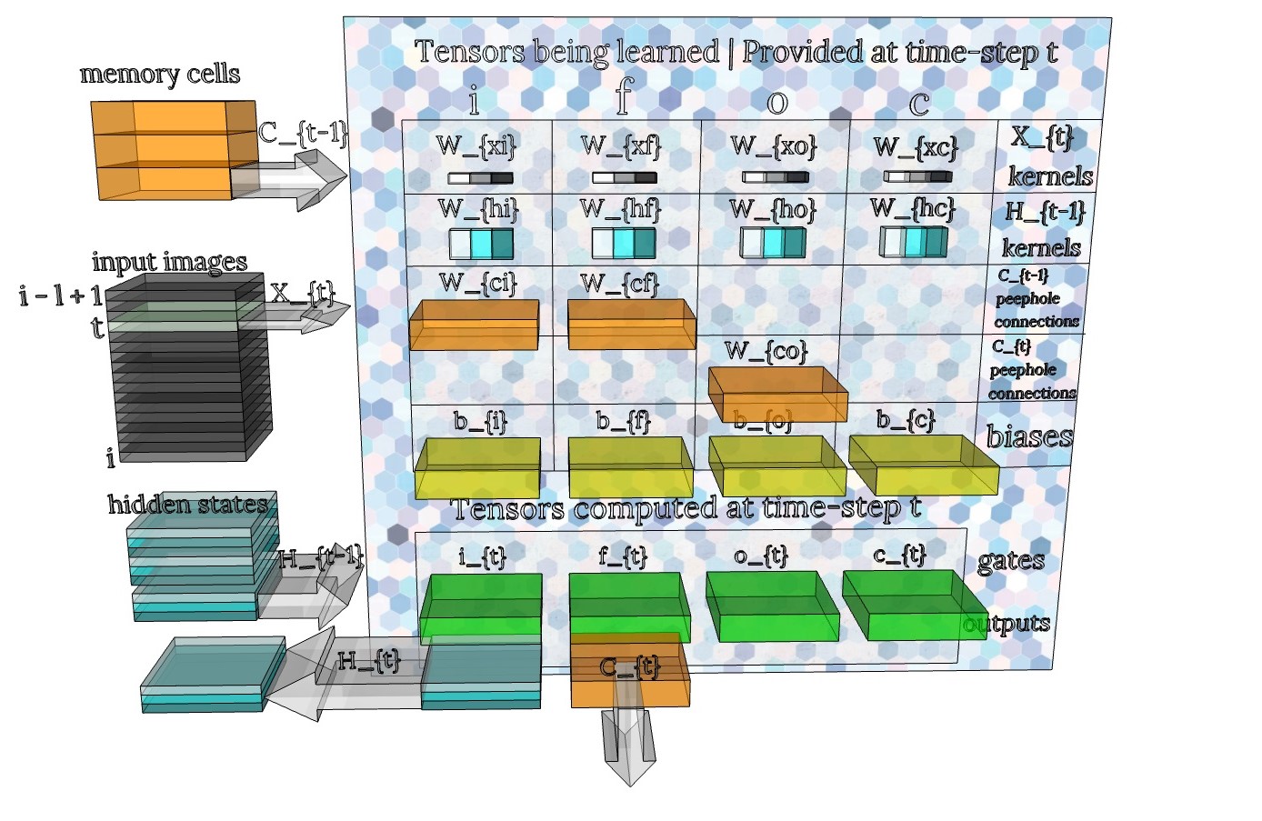 Fig ConvLSTM_Cell. Schematic for the ConvLSTM cell. The full input tensor \(X_i\) is shown as a stack of gray, single-channel images (rather than multi-channel images) for simplicity. In this particular illustration the ConvLSTM would have 3 “units” (ie 3 kernels). The corresponding channels of the hidden states are shown as a stack of 3 slices in 3 different shades of blue. At one time-step, image \(X_t\) and hidden state \(H_{t-1}\) are fed to the ConvLSTM cell. Convolution operations are performed on each tensor using the banks of kernels in the top two rows of the table. The results are added together and combined with the memory cell \(C_{t-1}\) and bias \(b\) to compute the gates \(i,f,o,c\) (green). Finally, the memory cell and hidden state are updated using the gates and are output for the next cycle. The process then repeats for the next image in the stack \(X_{t+1}\). I denoted the term \(tanh(W_{xc} * X_t + W_{hc} * H_{t-1} + b_c)\) as the gate \(c_t\). In LSTMs this gate is sometimes called the \(g\) gate.
Building the full model
Note: The model described in this section is called “visionary-serenity” (orange curve) in the figures in part 5
My full model consists of two stacked ConvLSTM layers (with max pooling and batch norm in between), followed by a global max pool, and finally a dense layer that outputs one probability value. The keras functional API code is below. The convLSTM_1 layer has return_sequences=True so that the hidden state \(H_t\) at each time-step is output. The whole sequence of \(H_t\) is then given as input to the next layer. I use the keras.layers.TimeDistributed wrapper to apply max pooling (and batch normalization) to each element in this sequence individually. Next, the convLSTM_2 layer has return_sequences=False so that only the very last hidden state is output. I then collapse the spatial dimensions of this tensor, taking only the max value in each channel. Finally I feed the resulting vector z to a dense layer.
Instead of using global max pooling, one could imagine flattening the output of convLSTM_2. My rationale is that we only want to detect the presence (not location) of features produced using the last convLSTM_2’s filters. Simply flattening the tensor would produce a vector which preserves information on the spatial locations of features, and this may not be totally necessary for classification purposes. Flattening also creates a vector with very high dimensionality and the dense layer immediately following it would thus require a huge number of parameters, slowing training time and limiting memory even further.
I had tested versions of the model where up to 4 ConvLSTM layers were stacked. But I could not get models with greater than 2 ConvLSTM layers to reach good performance. It is always good practice to start with smaller models and scale up if the model is learning good representations.
pooling_layer = tf.keras.layers.MaxPool2D(pool_size=(2, 2), padding='valid', data_format='channels_last')
batch_norm_1_layer = tf.keras.layers.BatchNormalization(axis=-1, center=False, scale=False, name='batchnorm_1')
L1L2 = tf.keras.regularizers.L1L2(l1=0, l2=0)

inputs = Input(shape=clip_tensor_shape)
convLSTM_1 = ConvLSTM2D(16, 3, strides=(1, 1), padding='valid', data_format='channels_last', activation='tanh',
                        recurrent_activation='hard_sigmoid', use_bias=False, return_sequences=True, return_state=False,
                        dropout=config.dropout, kernel_regularizer=L1L2,
                        name='convLSTM_1')(inputs)
max_pool_1 = TimeDistributed(pooling_layer)(convLSTM_1)
batch_norm_1 = TimeDistributed(batch_norm_1_layer)(max_pool_1)

convLSTM_2 = ConvLSTM2D(32, 3, strides=(1, 1), padding='valid', data_format='channels_last', activation='tanh',
                        recurrent_activation='hard_sigmoid', use_bias=False, return_sequences=False, return_state=False,
                        dropout=config.dropout, kernel_regularizer=L1L2,
                        name='convLSTM_2')(batch_norm_1)

z = tf.keras.layers.GlobalMaxPool2D(data_format='channels_last')(convLSTM_2)
y = Dense(1, activation='sigmoid')(z)

model = Model(inputs, y)

L = tf.keras.losses.BinaryCrossentropy(name='binary_crossentropy_in_loss')
model.compile(loss=L,
              optimizer=keras.optimizers.Adam(learning_rate=0.00008, beta_1=0.9, beta_2=0.999, amsgrad=False),
              metrics=[tf.keras.metrics.BinaryCrossentropy(name='binary_crossentropy_in_metrics'), tf.keras.metrics.AUC()])
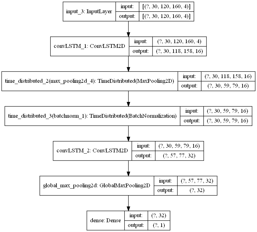 Fig. Final Keras model diagram. This is the model called “visionary-serenity” (orange curve) in the figures in part 5
Things that can affect the model’s ability to learn
I mentioned in part 1 that I had a tremendous amount of difficulty getting the model to learn good representations at all. The model could overfit easily on the training set, but it would remain at a validation ROC-AUC of 0.5 over several epochs. I tried adjusting the factors listed below. Ablation studies could help determine which was most critical to the model’s ability to learn, but I decided not to perform any.
I believe that performing data augmentation was essential; it allowed the validation AUC to grow above 0.5 for the first time.
All these factors can have an impact on the model’s ability to generalize to the test set:
- learning rate: a smaller learning rate worked better
- batch size: a batch size of 4 seemed to help. The memory constraints of this model also limit batch size.
- model size: In my case a smaller model worked better.
- class imbalance in the dataset. Use class weights or sampling strategies to ameliorate this.
- type and amount of regularization: I found L1L2 regularization had a powerful effect on overfitting, even with low strength parameters.
- data augmentation
- form of the input tensor (e.g. single-channel vs time-channels version of the input)
Training
With data augmentation, each epoch of the training set took 5h 16m on an NVDIA RTX 2080Ti GPU. I trained the model for 9 epochs, totaling 47 hours 25 min. The minimum validation loss occurred on the 4th epoch and the max validation AUC on the 6th. In the Github repository, I included the two best models in terms of validation loss: checkpoint_tc-augm-best-validation-retarget-no-regr-visionary-serenity (2nd best, 2-layer) and checkpoint_tc-augm-best-validation-retarget-upbeat-snowflake-91 (best, 1-layer). “visionary-serenity” is the model described in this section but a simplified version “upbeat-snowflake-91,” was used in all results figures.
| Training Dataset | Loss | Batch size | Optimizer | input size | regularizers |
|---|---|---|---|---|---|
| 44956 grayscale 120x160x1 images, augmented 4x | Binary Crossentropy | 4 | Adam, learning rate = 0.00008 | (30,120,160,4) |
None |