- part 1: An introduction to this project and links to the github repository.
- part 2: A list of subtasks involved with this project.
Experimental Setup
I transferred my 6 Serpae tetra fish from their home tank to the clean observation tank shown below. The walls of the observation tank have dots placed about 1 inch apart to act as a visual aid; the tank is otherwise completely white plastic. It was imperative to allow the fish to acclimate to this new environment for at least 24 hours; their behavioral pattern becomes dramatically more timid when initially introduced. Aggressive behavior resumed after the acclimation period.
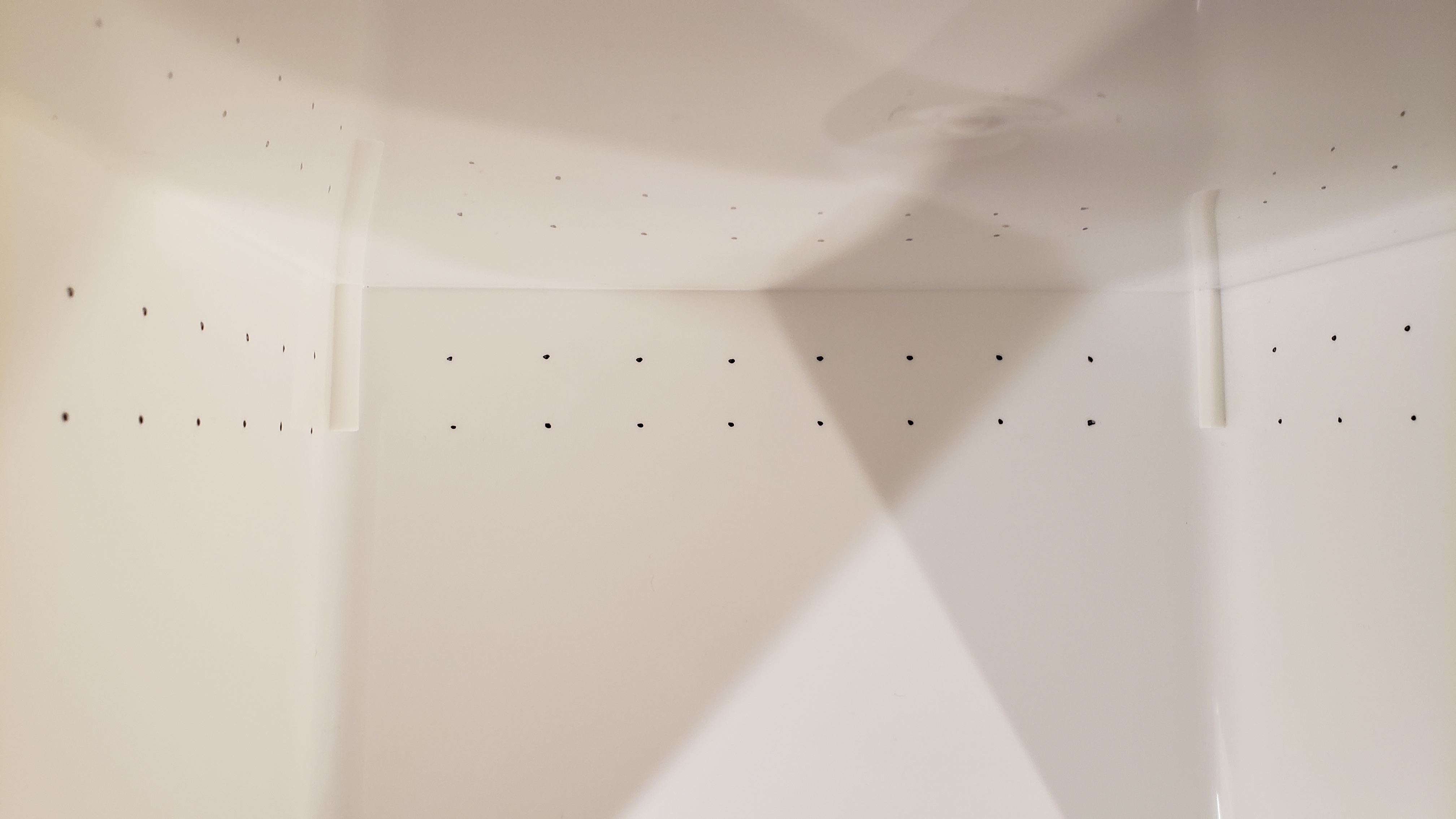 Fig. Fishes’ viewpoint from inside the observation tank.
I placed a DSLR camera overhead of my fish observation tank and recorded at 30fps for 30 mins while I was not in the room, at constant ambient temperature and light.
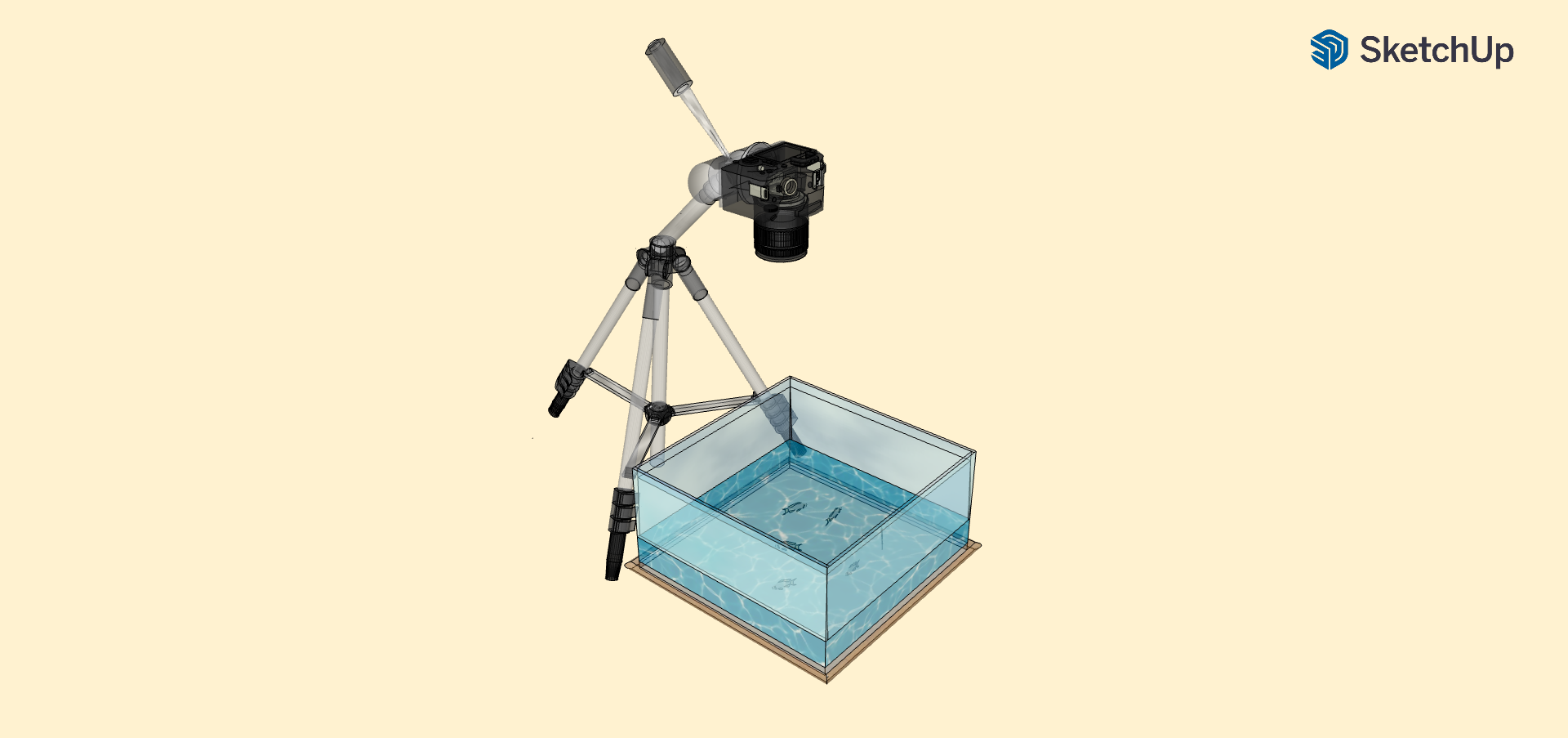 Fig. Video recording of observation tank
Footnote: [My Serpae tetra fishes’ behavioral style is extremely sensitive to changes in environmental conditions. They grouped very tightly, stopped moving, and ceased all aggressive behavior towards each other when initially introduced to the new tank. I increased the density (#fish/unit volume) by moving a sliding wall and this further increased the frequency of chasing behaviors.]
The Dataset
After image processing, converting from video to images, and down-sampling, I obtained a dataset of ~54000 grayscale images with 120x160x1 resolution.
| dataset | # images | % of total | length(min) | memory(MB) |
|---|---|---|---|---|
| training | 44956 (86.6% labeled negative) | 83.38 | 24.98 | 130 |
| validation | 3593 | 6.66 | 2 | 9.76 |
| testing | 5367 | 9.95 | 2.98 | 16.3 |
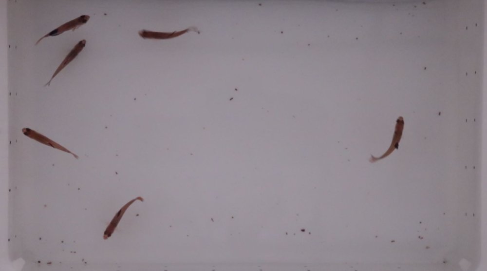 Fig. Unprocessed Video frame
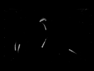
Fig. Processed video frame. An example of the images given to the model
Data augmentation
The training data was augmented at train time using horizontal and vertical flips, resulting in a 4x increase in the number of images. The augmented dataset contained the equivalent of 1h 40m of footage. Note that this type of ‘flipping and rotation’ augmentation will not necessarily be helpful in all tasks or datasets. The symmetries in my images made it extremely helpful—necessary even.
The augmentation was performed totally using the tf.data.Dataset method .map(). The relevant parts of the code to do augmentation of the training dataset ds_train are shown below for reference. In the later section “The input data generator” I describe how to create the python data generator passed into tf.data.Dataset.from_generator.
ds_train = tf.data.Dataset.from_generator(
    tc_inputs_generator,
    args=[start_frame_tr, end_frame_tr, training_dir, Y_label_train],
    output_types=(tf.float32, tf.int32),
    output_shapes=(clip_tensor_shape, ()))

ds_train_flip_HV = ds_train.map(lambda x, targ: (tf.image.flip_up_down(tf.image.flip_left_right(x)), targ))
ds_train_flip_H = ds_train.map(lambda x, targ: (tf.image.flip_left_right(x), targ))
ds_train_flip_V = ds_train.map(lambda x, targ: (tf.image.flip_up_down(x), targ))

# concatenate datasets:
ds_train = ds_train.concatenate(ds_train_flip_HV).concatenate(ds_train_flip_H).concatenate(ds_train_flip_V)
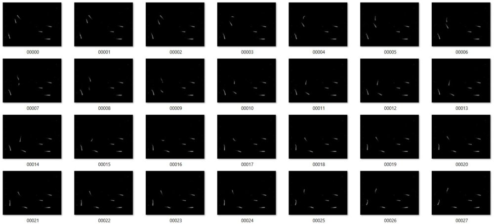
Fig. Sample of images from validation set. Images in the training and test set have the same file name format, with the first frame being 00000.png
Input Tensors
The input to this model is an ordered stack of video frames representing a 4 seconds video clip. I tried training the model using two versions of this tensor, called “single-channel” and “time-channels.” Only the time-channels version produced good accuracy on the test set so I will focus on defining that version. The single-channels tensor containing \(l\) images is simply a stack of images of shape (l, height, width, 1). The very last frame, at the top of the stack, is seen as the “current” frame.
The time-channels tensor is so-called because we allow each time-slice in the input tensor to be a stack of 4 grayscale images, each corresponding to one video frame. This is a similar idea to that used in Playing Atari with Deep Reinforcement Learning by DeepMind.
For the experiments in this paper, the function phi… applies this preprocessing to the last 4 frames of a history and stacks them to produce the input to the Q-function -Mnih et al. 2013
I use the parameter \(n=30\) to define the number of images or slices in the tensor. The final tensor has shape (n, height, width, 4) = (30, 120, 160, 4) where the first dimension represents time (and the channels dimension also represents time). There is no overlap between the 30 slices. Thus this tensor covers 30*4 = 120 frames = 4 seconds. I chose 120 frames as the length of video clip based on a combination of balancing memory constraints with capturing enough of the prior dynamics. 120 frames seemed to work heuristically.
In terms of indexing, the tensor for frame \(i\) contains the prior 120 frames: \(i \in [i - 4n + 1, i]\).
Defining the valid range of time points to sample from
Since each tensor covers 120 frames, we can’t sample an input tensor from the very first 120 frames. We must define a valid range of frames to sample from.
The valid range is \(i \in [4n - 1, T - 2 - h]\)
where \(i\) is the frame index in a 0-based indexing system. That is, the training set (and val and test) runs from image \(i=0\) to \(i=T\). The parameter \(h\) (defined later) is used by the labeling algorithm that produces ground truths for each frame in the valid range.
The input data generator
The best way I found to generate these input tensors in Keras-tensorflow was to use write my own python generator that would assemble images from the training or validation directory into tensors of the correct shape. It is called tc_inputs_generator in train_ConvLSTM_time_channels_with_augmentation.py. I then used tf.data.Dataset.from_generator(tc_inputs_generator,...) to create the tf.data.Dataset object that is actually passed to model.fit().
Since two consecutive input tensors have a large overlap, assembling inputs on-the-fly like this is important for memory-saving purposes. You wouldn’t want to save each individually as there would be a huge amount of redundant data.
In the following targets is an array of ground truth labels (either 0 or 1 for each tensor).
def tc_inputs_generator(t_start, t_end, image_folder, targets):
    t = t_start
    while t <= t_end:
        clip_tensor = []
        for j in range(t - 4 * n + 1, t + 1, 1):
            pil_img = load_img(image_folder.decode('UTF-8') + f'{j:05}' + '.png', color_mode='grayscale',
                               target_size=target_size)
            clip_tensor.append(
                img_to_array(pil_img, data_format='channels_last', dtype='uint8').astype(np.float32) / 255)
        clip_tensor = np.array(
            clip_tensor)  # concat all 4n clip frames along time axis. output shape = (4n, height, width, 1)
        clip_tensor = np.transpose(clip_tensor,
                                   axes=(3, 1, 2, 0))  # permute dims so tensor.shape = (1, height, width, 4n)
        clip_tensor = np.array_split(clip_tensor, n,
                                     axis=3)  # returns a list of n tensors, each with shape=(1, height, width, 4)
        clip_tensor = np.concatenate(clip_tensor,
                                     axis=0)  # finally concat along time axis, producing shape (n, height, width, 4)
        yield clip_tensor, targets[t]
        t += 1
Computing targets
As I described in part 2, we need a way to label each tensor/frame in the valid range as 0 or 1. This is too tedious to do by hand. I instead applied the ideas of self-supervision to label each video clip tensor:
I leverage the fishes’ future dynamics (in frames \(i\) to \(i+h\); \(h=45=1.5 s\)) to label the video clip encompassing the past 120 frames (4 s).
Computing the mean speed proxy \(\tilde{y}\)
Specifically, for each consecutive pair of frames \((i, i+1)\) I compute a proxy for the group mean swimming speed called \(\tilde{y_i}\). \(\tilde{y_i}\) measures the absolute change in pixels between frames \(i\) and \(i+1\). The faster the fish move, the more pixels have changed between consecutive frames, and the higher is \(\tilde{y_i}\).
From the method compute_targets below, we take the sum of the absolute difference and normalize by the number of pixels:
y_tilde[t] = np.sum(np.abs(img_array_1 - img_array_0))/np.prod(img_array_0.shape)
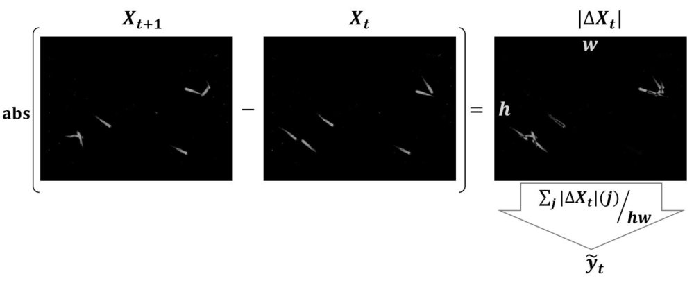 Fig. How \(\tilde{y_t}\) is computed. \(X\) represents an image, \(w\) and \(h\) are its width and height in pixels. The index \(j\) correponds to one pixel in the difference image \(\Delta X_t\).
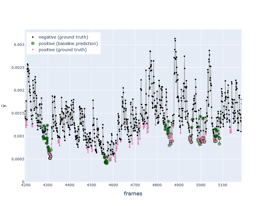
Fig. Zoomed section of \(\tilde{y_i}\) timeseries (in test dataset), with ground truth labels and predictions from the baseline algorithm (covered later) Pink points indicate the moment right before a spike in \(\tilde{y_i}\)
Ground truth labeling algorithm
After computing \(\tilde{y_i}\), the algorithm produces a label based on the dynamics of \(\tilde{y_i}; i \in [i, i+h]\).
The idea is to label frames as positive if they precede a sudden spike in mean swimming speed (indicated by \(\tilde{y_i}\)).
At this point it is important to highlight how the inputs to the labeling algorithm differ from the inputs to the model. This is at the core of how the problem is brought into a self-supervised setting. See the figure below.
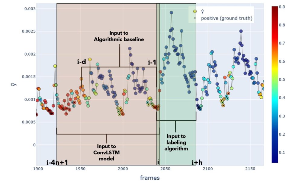 Fig. Input windows to each model or algorithm. Actual window sizes used in experiments are shown. Positive ground truth labels are shown as black dots, and the ConvLSTM-based model’s predicted probability is colorized. Y-axis indicates \(\tilde{y}\).
The rules I chose for labelling were found heuristically by inspecting the data in plots and trying different parameters. I’ll write it mathematically first, and then in code. See the figure below for illustration.
Let
\[W_i = \{\tilde{y_t}; t \in [i, i+h]\}\] \[R_i = range(W_i)\]Then, \(R_i \geq c \text{ AND } \tilde{y_i} \leq min(W_i) + bR_i \Rightarrow y_i \leftarrow 1\)
where \(i\) is the frame being labeled, \(h=45\) frames, \(c=0.001\), and \(b=0.1\).
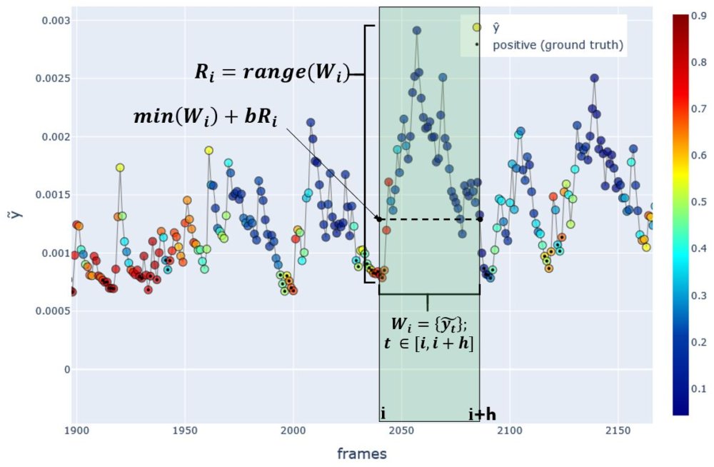 Fig.H Method for labeling each frame. Here the frame \(i\) is being labeled as \(y_i=1\) since it precedes a sudden rise in the speed proxy \(\tilde{y}\). Color indicates the model predictions \(\hat{y}\). Frames with a circled dot represent positive ground truth \(y_i=1\), and without dot represents negative \(y_i=0\).
Now in the python code, I label a frame t as 1 if
y_tilde[t]is low (relative to the values iny_tilde[t:t+h+1]) (ie \(\tilde{y_i} \leq min(W_i) + bR_i\)) ANDy_tilde[t:t+h+1]has a range that exceedsc,
and label as 0 if it did not meet these conditions. The parameters b and c obviously affect the number of positively and negatively labeled frames.
    b=0.1
    c=0.001
    y_label = np.zeros(T)
    for t in range(tc_start_frame, tc_end_frame+1):
        if np.ptp(y_tilde[t:t+h+1]) >= c and y_tilde[t]<=(np.min(y_tilde[t:t+h+1])+b*np.ptp(y_tilde[t:t+h+1])):
            y_label[t] = 1
Finally, putting it all together:
def compute_targets(image_folder):
    T = count_files(image_folder)
    tc_start_frame = 4 * n - 1  # first frame inded in the valid range
    tc_end_frame = T - 2 - h  # last frame index in the valid range, assuming images start at t=0 and go to t=T-1
    y_tilde = np.zeros(T)
    for t in range(T-1): #T-1
        pil_img_t0 = load_img(image_folder+f'{t:05}' + '.png', color_mode='grayscale', target_size=None)
        pil_img_t1 = load_img(image_folder+f'{t+1:05}' + '.png', color_mode='grayscale', target_size=None)

        img_array_0 = img_to_array(pil_img_t0, data_format='channels_last', dtype='uint8')
        img_array_1 = img_to_array(pil_img_t1, data_format='channels_last', dtype='uint8')
        #we must convert to float32 before performing subtraction, otherwise all negative values will be set as 255
        img_array_0 = img_array_0.astype(np.float32)/255
        img_array_1 = img_array_1.astype(np.float32)/255

        y_tilde[t] = np.sum(np.abs(img_array_1 - img_array_0))/np.prod(img_array_0.shape)#Also must normalize by numbr of pixels

    # label each frame algorithmically
    b=0.1
    c=0.001
    y_label = np.zeros(T)
    for t in range(tc_start_frame, tc_end_frame+1):
        if np.ptp(y_tilde[t:t+h+1]) >= c and y_tilde[t]<=(np.min(y_tilde[t:t+h+1])+b*np.ptp(y_tilde[t:t+h+1])):
            y_label[t] = 1

    return y_tilde, y_label
The algorithmic baseline
For the sake of time I won’t go into detail on the algorithmic baseline; it may be more easier to just take a look at the function: baseline_prediction_probabilistic in my notebook Compute_targets-time-channels.ipynb. The algorithm works only with \(\tilde{y_i}\) data as input and, for each frame, outputs a probability it was labeled as 1. It uses a very similar technique as the ground truth labeling algorithm compute_targets, except that it uses a window over past frames y_tilde[t-d:t] where d=89 to predict the label of the frame t. Notice that the window y_tilde[t-d:t] does not contain the point y_tilde[t] (due to in python’s indexing system), so we are not using any information about the current or future states to predict the current state.