- Notice: Please see part 1 for an introduction to this project.
- Repository for this project: Github
- python file for training ConvNet:
FCN512_2.py - Jupyter notebooks used for image learning and plots:
Learn_image.ipynb,Generate_plots.ipynb
In Brief
- In deep generative modeling, Texture synthesis is the process of creating novel texture images. Texture extraction involves taking a natural image and producing images with qualitatively similar texture properties.
- In this project, I develop a novel texture extraction model that uses image-learning-based techniques. This make it similar to something like the original neural style transfer process. However, I employ a texture descriptor based on global average pooling across convolutional channels. This descriptor effectively captures how all convolutional filters in a (pre-trained) fully convolutional network (FCN) are activated. I first train a generative FCN (structured like an autoencoder) on a lichen photo dataset that I created. I then iteratively optimize a texture image until its texture descriptor vector matches that of a target image.
- Research question: 1. How does my novel texture descriptor perform?–what will the synthetic images derived from it look like? 2. What effect does the FCN’s training data have on the textures generated?
- Result: When learning a new texture image, my model captures the color distribution of the target image well. The spatial features in the learned image do not reflect those in the target image very well. However, the nature of the training data had an obvious impact on the appearance of textures that could be generated.
- In part 1/2: I’ll give a broad overview of the different paradigms in deep generative modeling, as well as some alternative texture extraction models from the literature that had better performance. This is useful since it classifies my own model and contrasts it with fundamentally different methods such as GANs.
- In part 2/2 (this post): I’ll cover my dataset, network architecture, image learning algorithm, and results.
Research Objective
Is it possible to take a natural image and “extract” the textures within it? I.e Can we generate images containing new instances of those textures? This texture synthesis, or more specifically, texture extraction is one of many challenging computer vision tasks that has been advanced substantially in recent years by convolutional neural networks (CNNs). The authors of Learning Texture Manifolds with the Periodic Spatial GAN describe it this way
The goal of texture synthesis is to learn from a given example image a generating process, which allows to create many images with similar properties.
In this project I develop and evaluate a novel texture extraction method that is image-learning-based, meaning we optimize (learn) the pixel values of an image directly by iteratively applying gradients to the image. My procedure is in the same spirit as convolutional filter visualization, neural style transfer, or DeepDream.
I ask whether a novel texture descriptor based on global average pooling across all convolutional channels can capture qualitative features of the texture in a target image. I also ask how the original data that the network was trained on affect the textures that can be generated.
Brief Methods
There are two main steps in the pipeline. The first involves training a fully convolutional network (FCN), that is set up like an autoencoder, to take input texture images and reconstruct them. This forces the network to learn meaningful feature detectors (i.e. convolutional filters) that can later be used to represent the texture of a new image (that I call the “target” image).
The second step is to run the algorithm that, starting from an initial condition of noise, learns a new image \(Z\). The texture of the learned image \(Z\) is intended to match that of a target image \(A\). The learned image is iteratively updated in such a way that its texture descriptor (called the “global average pooling (GAP) vector” \(z\)) approaches that of the target image’s texture descriptor, \(a\). The GAP vectors are computed by sending an image through the FCN and individually pooling the feature maps at all convolutional layer channels (See Figure GAP). After image learning, when fed into the FCN, Z should activate the network’s filters in a similar way as A.
In the next sections I’ll first cover the dataset and training process for step 1, and then explain the texture extraction algorithm.
Dataset
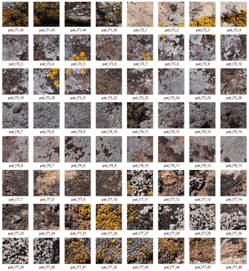
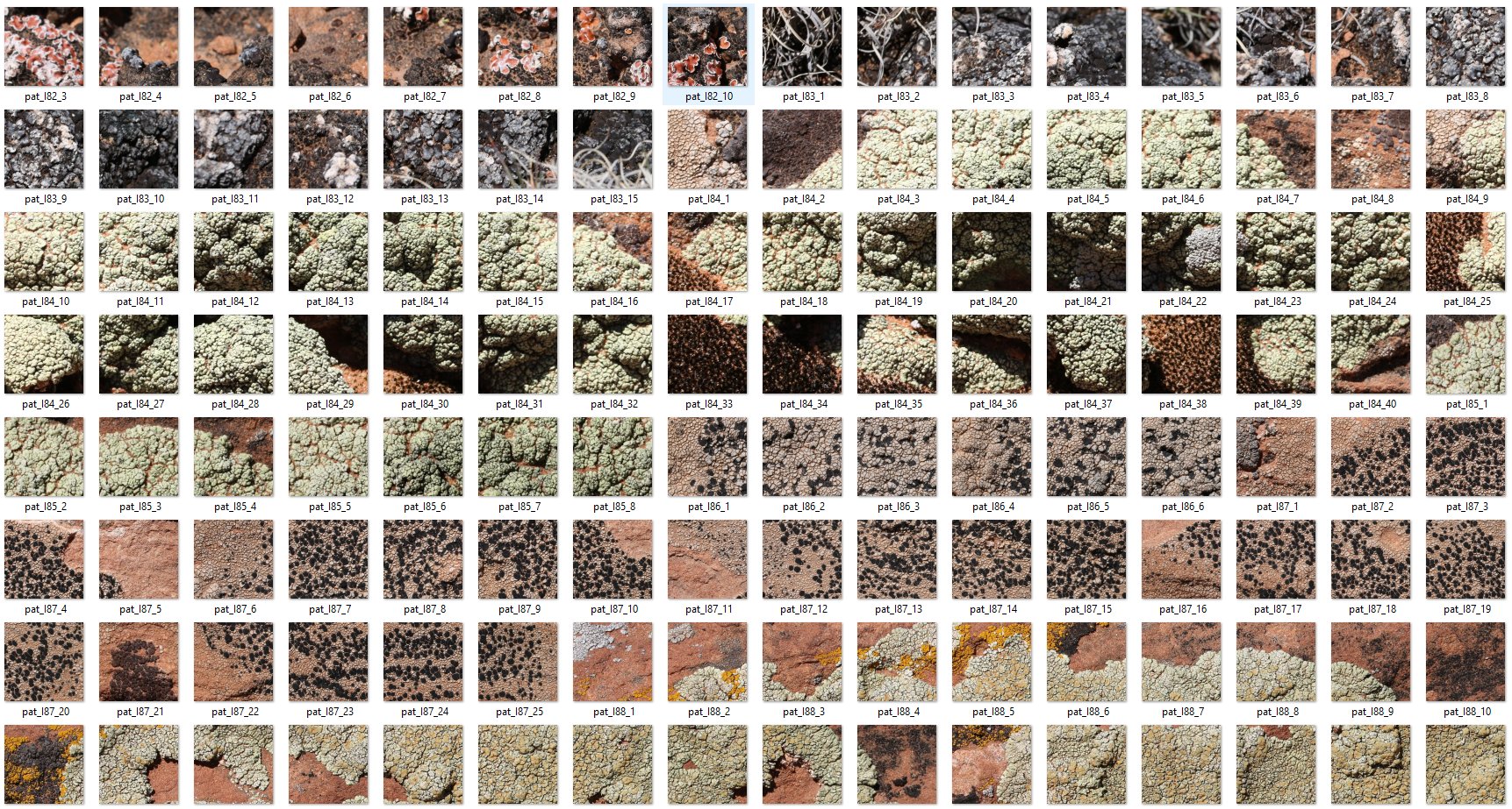
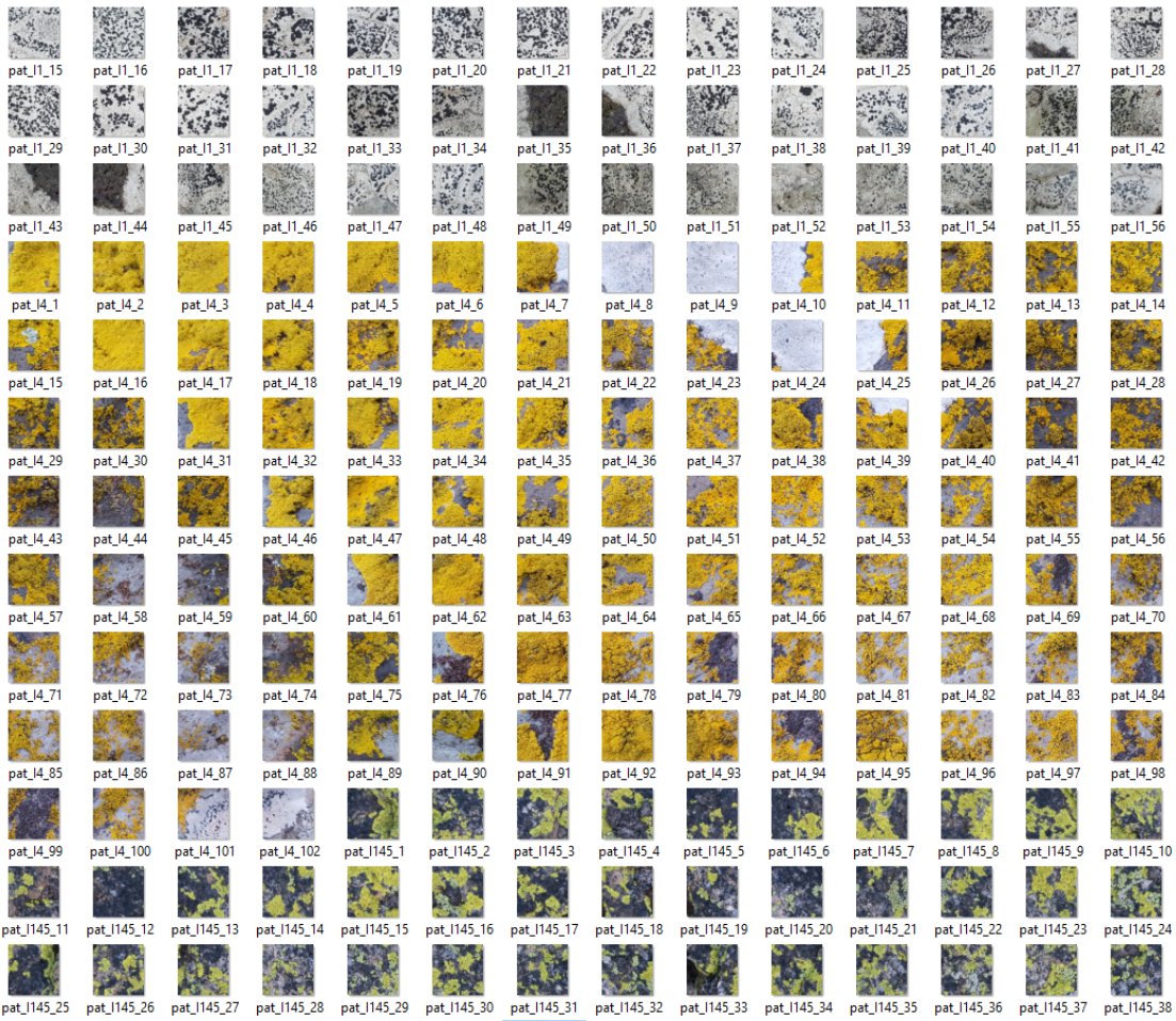
I constructed the training data from 148 macro photos of lichen that I had taken while travelling across the United states (mostly Arizona and Washington). In order to focus on textures, each training image was partitioned into some number of non-overlapping square sub-images with sizes ranging from ~300x300 to ~600x600. During training all were resized to 512x512x3 pixel patches, for a total of 4323 patches (1.92GB). I did not use any data augmentation but rotating by multiples of \(90^\circ\) would be reasonable for these type of images. Screenshots of the patches are below.
Fully convolutional net architecture and training
The FCN is trained exactly like an autoencoder. Batch gradient descent is used to minimize the mean squared error between the pixels of the input image and the reconstructed output image. A key difference here is that there are no pooling layers. For the end-purposes of this model, there does not seem to be a reason to compress the input information through a bottleneck. I kept the same spatial dimensions all the way through for simplicity. This network does not just learn an identity mapping, where the image is copied over and over until the output. As we will see later, the convolutional filters learned have a great impact on the textures that can be generated. Below you can find more details on the layers such as kernel sizes and strides.
FCN_input = keras.Input(shape=(512, 512, 3), name='FCN_input')
x = layers.Conv2D(32, 7, strides=(1, 1), activation='relu', padding='same')(FCN_input)
x = layers.Conv2D(32, 7, strides=(1, 1), activation='relu', padding='same')(x)
x = layers.BatchNormalization(axis=-1)(x)
x = layers.Conv2D(64, 5, strides=(1, 1), activation='relu', padding='same')(x)
x = layers.Conv2D(64, 5, strides=(1, 1), activation='relu', padding='same')(x)
x = layers.BatchNormalization(axis=-1)(x)
x = layers.Conv2D(64, 3, strides=(1, 1), activation='relu', padding='same')(x)
x = layers.Conv2D(64, 3, strides=(1, 1), activation='relu', padding='same')(x)
x = layers.BatchNormalization(axis=-1)(x)
x = layers.Conv2D(64, 1, strides=(1, 1), activation='relu', padding='same')(x)
x = layers.Conv2D(64, 1, strides=(1, 1), activation='relu', padding='same')(x)
x = layers.BatchNormalization(axis=-1)(x)
FCN_output = layers.Conv2D(3, 1, strides=(1, 1), activation='relu', padding='same')(x)
FCN = keras.Model(FCN_input, FCN_output, name='FCN')
| Dataset | Loss | Batch size | Optimizer | input size | # parameters |
|---|---|---|---|---|---|
| 4323 RGB images, 1.92GB | Mean squared error. Unsupervised training (ground truth = input) | 8 | Adam, learning rate = 0.001 | 512 x 512 x 3 | Trainable: 148387, Non-trainable: 448 |
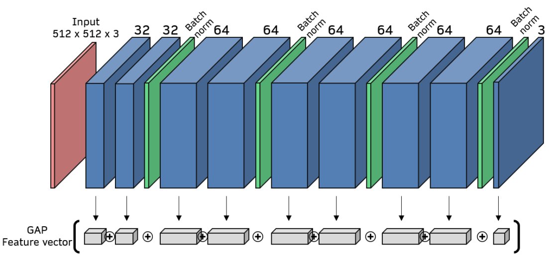 Fig GAP. FCN architecture and GAP feature vector. Blue boxes are convolutional layers and green are batch norm layers. NOTE: batch norm layers are drawn as thin slices to save space, but their output has the same shape as the preceding layer. The GAP vector is taken by performing global average pooling of all convolutional layer channels. This produces one vector element per channel. The full vector is a concatenation of all such GAP values.
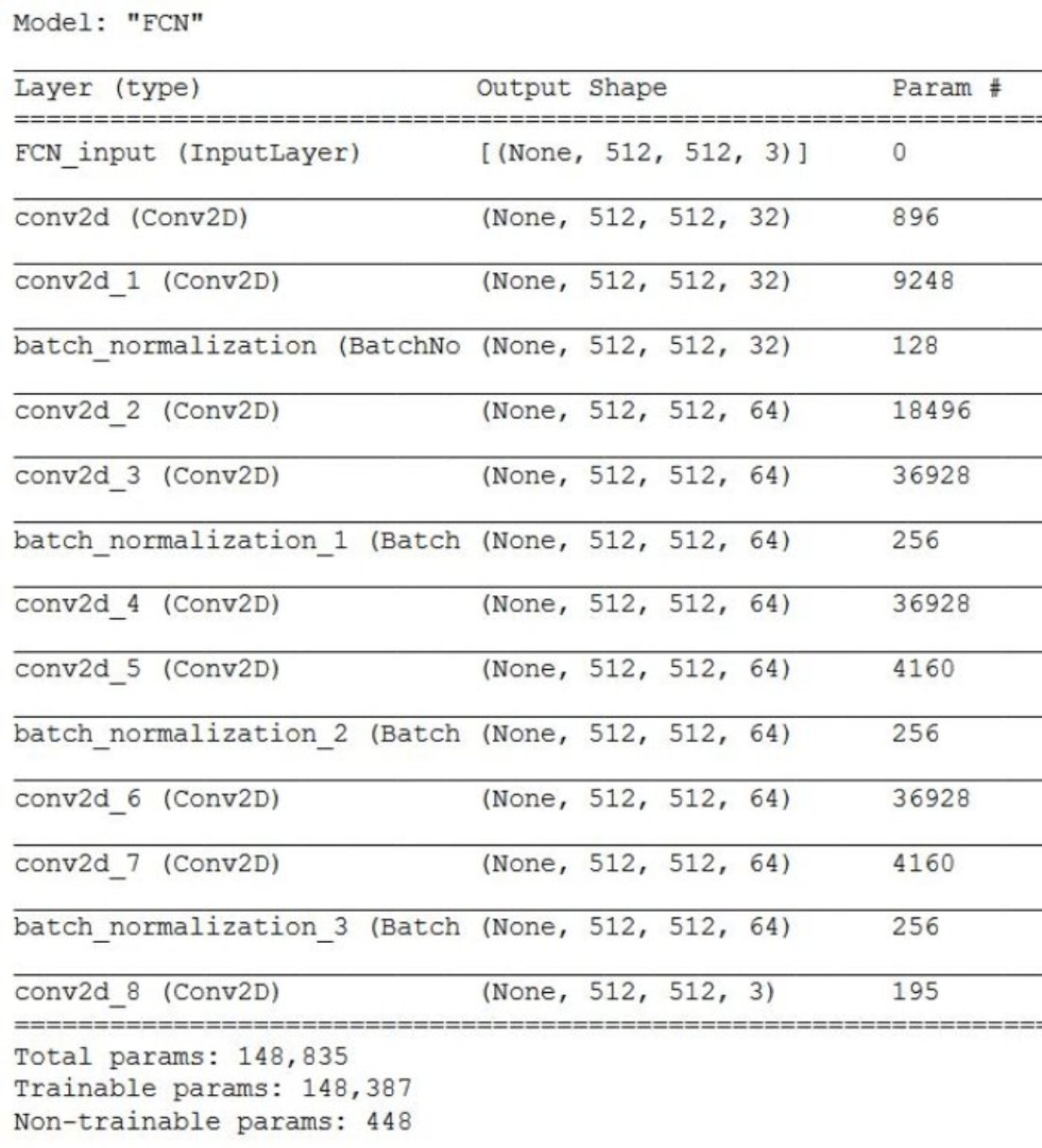 Fig. Tensorflow model summary
Image-learning Algorithm
The trained FCN model will be denoted as a function \(F\), and its output at layer \(l\) is denoted \(F^{(l)}(X)\), where \(X\) is an input image. \(F^{(l)}(X)\) is a tensor containing \(d^{(l)}\) feature maps. I equivalently call it \(Y^{(l)} \equiv F^{(l)}(X)\). For each \(Y^{(l)}\), we compute the GAP vector segment \(g^{(l)} \in \mathbb{R}^{d^{(l)}}\) by taking the average of all pixels in each channel. This happens in the function called “GAPL()” in the Algorithm 1 below. Then, the function “GAPVector()” in Algorithm 1 simply concatenates all layers’ \(g^{(l)}\), resulting in the full GAP texture descriptor.
The texture extraction process is framed in my case as an image optimization problem. We compute a loss \(L\) based on the mean squared error between the GAP descriptors \(z, a\) of learned image \(Z\) and target image \(A\). I ran the for loop for n=15 iterations. By that point, the learned image had more or less stabilized. At each iteration gradient descent of the loss function is performed by subtracting a gradient tensor \(\nabla_{bfgs}L(Z)\) from \(Z\). Note that this gradient is the exact same shape as \(Z\). \(\nabla_{bfgs}L(Z)\) denotes the gradient of the loss function with respect to the pixel values in \(Z\). This gradient is computed using the Limited-memory BFGS optimization algorithm. After the gradient is applied, we send the new image through the network and re-compute its descriptor \(z\). The cycle then repeats (See Algorithm 1).
| Symbol | Meaning |
|---|---|
| Z | learned image |
| A | target image |
| z | full GAP descriptor for Z |
| a | full GAP descriptor for A |
| \(Y^{(l)}\) | all feature maps for layer l |
| \(F^{(l)}(X)\) | the model’s output at layer \(l\), given input image \(X\). (Equivalent to \(Y^{(l)}\)) |
| L | loss value |
| \(g^{(l)}\) | GAP vector for layer l |
| \(l\) | layer index |
| \(d^{(l)}\) | # channels in layer l |
| m | # layers in network |
| \(\nabla_{bfgs}L(Z)\) | gradient of loss w.r.t. Z from bfgs algorithm |
| \(Z_{noise}\) | noise image with same size as Z (initial condition) |
| \(h^{(l)}\) | feature map height spatial dim |
| \(w^{(l)}\) | feature map width spatial dim |
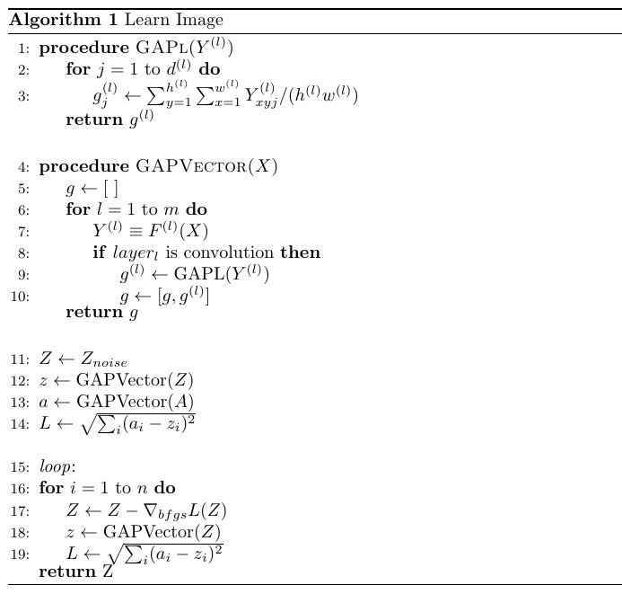
Fig. Algorithm pseudocode
Excerpt from Learn_image.py
outputs_dict = dict([(layer.name, layer.output) for layer in FCN.layers[1:]]) # creates a dict of layer outputs that can be easily accessed to get intermediate outputs

def get_GAP(layer_output):
    #input is a (height, width, channels) tensor. We first permute_dimensions to (channels, height, width). Then take the sum over all pixels in each channel.
    #each element j of the output is the mean across all pixels in the channel j
    return K.mean(K.batch_flatten(K.permute_dimensions(layer_output,(2,0,1))), axis=1)

GAP_target_img = []
GAP_learned_img = []

# cycle through all non-batch norm layers and concat the GAP into one long vector with length equal to the number of channels in the entire network
for name in outputs_dict:
    if name.find('batch_normalization') == -1: # skip batch norm layers
        layer_features = outputs_dict[name]
        GAP_target_img.append(get_GAP(layer_features[0]))
        GAP_learned_img.append(get_GAP(layer_features[1]))

GAP_target_img = K.concatenate(GAP_target_img, axis=0)
GAP_learned_img = K.concatenate(GAP_learned_img, axis=0)
GAP_learned_img

Loss = K.sqrt(K.sum(K.square(GAP_target_img-GAP_learned_img)))
grads = K.gradients(Loss, learned_image)[0]

fetch_loss_and_grads = K.function([learned_image], [Loss, grads])
Results and Discussion
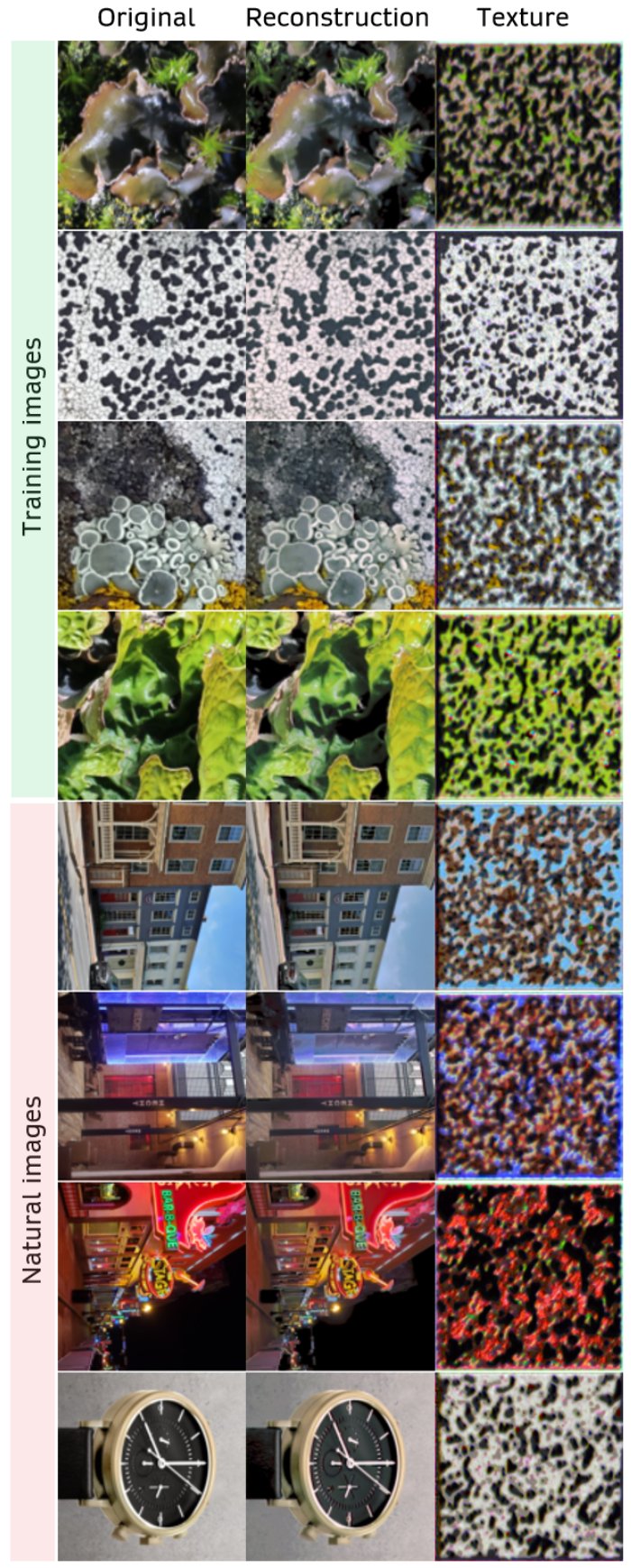
I first tested the ability of the trained FCN to reconstruct images. In the figure below, I passed both training images and natural images not from the lichen dataset through the model, and I found that both could be reconstructed well. While this certainly shows that that the model has not been overfit, it begs the question of whether the model has actually learned meaningful feature detectors. For example, the model might be performing an identity mapping in which the input is simply copied over and over. This is something I did not investigate yet. I believe that the lack of pooling layers prevented information from being lost, and this is part of the reason why the reconstructions are so close to the inputs.
In the figure below, I synthesized texture images from 4 training images and 4 natural images not from the training set. My algorithm optimizes an image such that it produces a similar GAP descriptor as a target image. Thus, the ‘Texture’ images appear the same, from the perspective of the GAP descriptor, as the ‘Original’ images. Since each vector element of the GAP descriptor pools across the spatial dimensions of a channel, spatial information is lost. For this reason it’s impossible to recover more complex or larger scale structures seen in the training images.
Why do the textures look like that and not something else?
The textures synthesized are not random noise. They are not arbitrary—there is a specific reason they look this way.
Each element of the GAP vector measures only the degree to which a particular filter was activated. In other words, a higher value at \(z_j\) indicates greater presence of the image feature detected by filter \(j\). The visual appearance of the texture is thus heavily influenced by the types of image features that the network saw during training. For example, if you were perform the same process using VGG net trained on the imagenet dataset, the texture would look completely different. In summary, the textures produced by my network look vaguely like the lichen images it was trained on, and this makes sense. You are asking a network that has been trained to detect certain types of features to produce images containing those features.
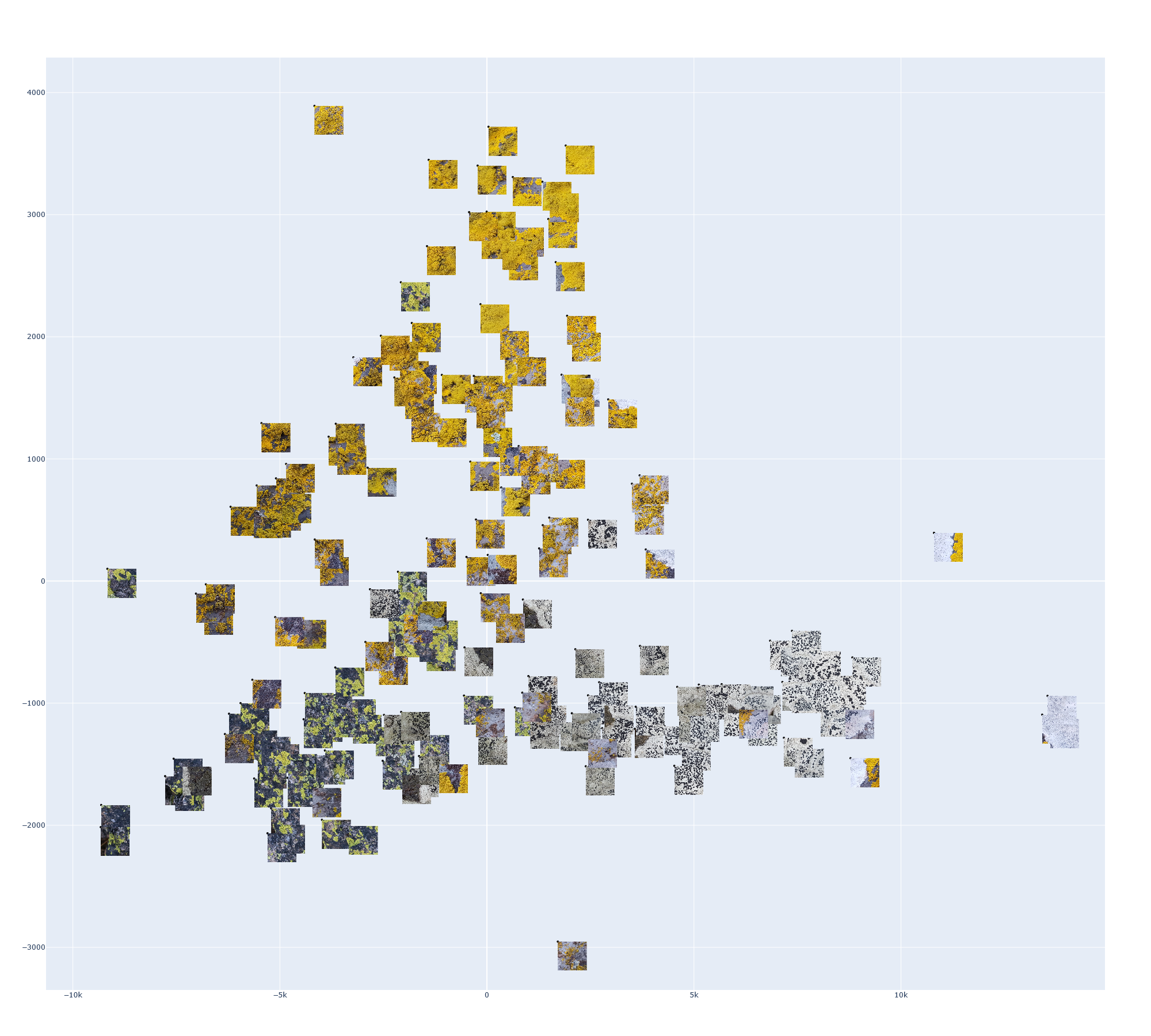
Using the GAP vector as a feature vector in clustering and dimensionality reduction
Finally, for the sake of testing its application as a feature vector, I performed t-SNE dimensionality reduction on a set of GAP vectors. The dataset (a subset of the training data), containing patches from three full-sized images is shown below. I embedded the GAP vector of each image into a 2D space and annotated each point with its patch. The code for this can be found in Generate_plots.ipynb
Thanks for reading!