Deep Audio Embedding

I use deep autoencoders to represent audio (music) as trajectories in a low-dimensional embedding space. My end-to-end architecture attaches a recurrent module to the output of the encoder. Its task is to predict the next point in the trajectory. This conditions the encoder to produce smoother trajectories than a traditional autoencoder would—a feature that might improve forecasting accuracy when modeling physical systems.

Project In Brief - TLDR

• Youtube video
• Temporal structure is inherent to all music but is often difficult to visualize in a space. I wanted to build a system that could represent the patterns in music in 3D.
• I created an autoencoder-based, end-to-end architecture that 1. embeds audio as a trajectory in a low-dimensional embedding space, 2. encourages the encoder network to produce smoother trajectories, and 3. forecasts the next time-step in embedding space. I asked what effect (2.) would have on forecasting accuracy, when compared with traditional autoencoders.
• The reason for including forecasting in the model is not because we’re interested in predicting how the music/audio will evolve. I found that music, once embedded, tends to look like a chaotic attractor. I thus treated my music embeddings as proxies for the dynamics of chaotic physical systems. Namely, I used them (simply as a data source) to prototype models that try to improve forecasting ability. The idea is that the model features developed could be useful when forecasting actual physical systems.
• Methods: I used Keras-tensorflow to develop my models. The datasets consist in multiple ~30s clips, each from a different piece of music. One model is trained from scratch per each song. The trained model is then used to embed the song it was trained on. Forecasting accuracy is compared between two versions of the model. One model is a pure autoencoder. The other is the same autoencoder but conditioned for better forecasting accuracy using an additional loss term.
• Result: In a sample of songs from diverse genres, most had similar limit-cycle-like structures when embedded using my method (essentially, a noisy loop, often with multiple “lobes”). In these cases, the model revealed rhythmic sequences that could be heard best in the drums. For songs where this did not occur, the embedding is more complex. My model produces significantly smoother embeddings than a pure autoencoder. However, this only improves forecasting accuracy on a short time scale.

GitHub Repositories

GitHub – Deep-Audio-Embedding

1. Convert a .wav file to spectrogram and save variables
   • Save-dataset_2sec-window.py – Saves spectrogram and other variables needed for step 2. compatible with the 2s sliding window model.
   • Save-dataset_half-sec-window.py – Saves spectrogram and other variables needed for step 2. compatible with the 0.5s sliding window model.
2. Build and train model on the audio from step 1.
   • Train_model_2sec-window.py – Trains a model that takes a 2s window from the spectrogram as input
   • Train_model_half-sec-window.py – Trains a model that takes a 0.5s window from the spectrogram as input
3. Load trained model. Extract encoder network. Feed spectrogram data to it and return embedding.
   • Embed_audio_data_callable.py – this is called at the end of Train_model...py. It also plots the embedding in 3D.
4. Plot video of embedding
   • Play_embedding.py – Saves a sequence of video frames where a point moves down the trajectory over time
5. Train models to forecast in embedding space using the embedding from step 3
   • train-latent-space-MLP.py – Trains an MLP regression model to predict the displacement vector from the position in the embedding space
   • train-latent-space-LSTM.py – Trains an LSTM-based regression model to predict the displacement vector from a sequence of positions in the embedding space
6. Use model trained in step 5 to forecast a path from some initial condition
   • Forecast-in-latent-space-KNN.py – Forecasts and plots a path in embedding space using a KNN-based method
   • Forecast-in-latent-space-MLP.py– Forecasts and plots a path in embedding space using the MLP trained in step 5
   • Forecast-in-latent-space-LSTM.py– Forecasts and plots a path in embedding space using LSTM trained in step 5
7. Measure divergence of numerical solutions from true path (using the KNN-based forecasting model)
   • Numerical-solution-divergence.py – Forecasts a path at a set of initial conditions. Measures distance between projected and actual path. Returns an average curve.
   • Numerical-solution-divergence-Plots.ipynb – Plots the divergence over the number of forecasting steps taken. This shows how fast error grows on average.

GitHub – Deep-Video-Embedding

1. Build and train model
   • train_model.py
2. Use trained model from step 1 to embed video as trajectory in embedding space
   • Embed-data.py
3. Plot video of embedding
   • Play_embedding.py – Saves a sequence of video frames where a point moves down the trajectory over time.
4. Train an LSTM-based model to forecast in embedding space using the embedding from step 2
   • train-latent-space-LSTM.py – Trains an LSTM-based regression model to predict the displacement vector from a sequence of positions in the embedding space
5. Forecast and plot a trajectory from a random initial condition in embedding space
   • Forecast-in-latent-space.py
6. Load forecasted trajectory from step 5 and plot over embedding in 3D
   • Plot-with-ZForecast.py
7. Evaluate performance of forecasting LSTM
   • Evaluate-LSTM-on-test.py – computes the mean squared error and mean cosine similarity between true and predicted displacement vectors in embedding space

Introduction

A principle underlying nearly all of data science is that objects comprising our world can be represented as feature vectors in some space. When representing a set of objects belonging to some group (e.g all chairs, all insects, or all trees), they typically have some non-uniform distribution in their features space. Another way of saying it is that these objects lie on some data manifold. Data manifolds are extremely common in nature, and I would argue that the concept is practically a statement of universality because it encapsulates so many diverse phenomena.

In this project, I was curious about how the data manifolds in music would appear. If we represented the flow of music as a trajectory through a feature space, what would it look like? Almost all music has some temporal structure, usually involving repetition of some parts and transitions between parts. Sometimes a section within a song is repeated while layers of instrumentation is incrementally added. How to properly visualize these transitions in a two or three-dimensional space is not obvious. The few examples that come to mind are sheet music or the track/instrument layouts in digital audio workstations (DAWs) like Pro Tools, Reason, or Garageband. These are very coarse representations at best. They don’t intuitively capture how music evolves and the similarities and differences among its parts.

I have two objectives for this work.

1. Reveal the trajectories corresponding to different pieces of music (in a 3D embedding space). I made videos synchronizing the audio with a point as it moves down the trajectory. This allows you to see (and hear) how the changes in sound affect the trajectory.
2. Develop a deep neural net that can simultaneously embed the audio and forecast the position of the next time-step in the embedding space. I force the encoder to produce an embedding that will later be used for forecasting (during training). This changes the embedding, relative to a pure autoencoder’s. I determine whether this change improved the accuracy of a predictive model trained on the embedding. (no it doesn’t really)

Related work

• Image Spaces and Video Trajectories: Using Isomap to Explore Video Sequences (paper)
• Discovering governing equations from data by sparse identification of nonlinear dynamical systems (SINDy paper)
• SINDy video, Steve Brunton
• My previous algorithm for mapping particle system dynamics into phase space (video)

Methods

Embedding pipeline

Fig. How raw audio gets embedded using the trained encoder network. A sliding window (green) moves across time in the spectrogram. At each position the data in the window is compressed to a single point in 3D.

To embed I first take a .wav file and convert it to a spectrogram using python’s scipy.signal. The .wav is read in an 1D array representing (time x amplitude) and the spectrogram is a 2D array (time x frequency). I move a sliding window of length 0.5s or 2s across the time axis of the spectrogram and, at each time-step, feed the window to the (trained) encoder network. The encoder represents the subimage \(x_t\) as a single point \(z_t\) in the embedding space \(\mathbb R^3\). I built a custom data generator to generate these windows (See inputs_generator_inference in Embed_audio_data_callable.py). The window moves forward by only 0.0232s each time-step. When using 0.5s windows, consecutive windows overlap by \(95.4\%\). \(z_t\) and \(z_{t+1}\) will thus be very close in the embedding space.

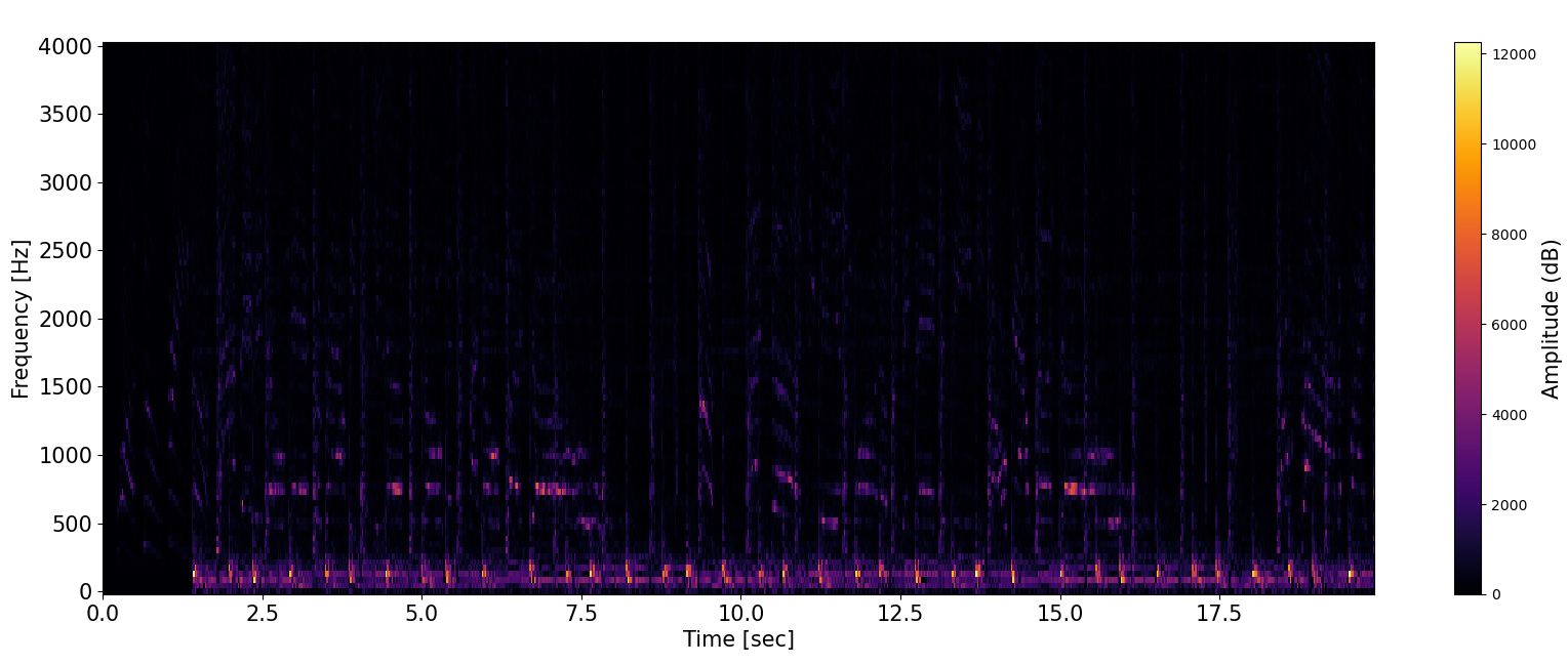Fig. Example spectrogram. X-axis indicates time (s) and Y-axis is frequency (Hz). Pixel intensity comes from the fourier transform and can be thought of as the degree to which each frequency is present in the audio signal at a certain time.

Conditioned Autoencoder model

Fig. Model inputs, architecture, and loss function at a high level.

At the core of my model is a deep convolutional autoencoder which takes in a window \(x_t\) from the spectrogram, represents it in embedding space as a vector \(z_t\), and reconstructs it as \(\hat{x_t}\). We feed two separate inputs the the encoder: 1. a stack of \(l\) consecutive windows and 2. a stack of two consecutive windows. Stack 2 contains the window \(x_{t+1}\), which is not included in stack 1.

We then compute the “true” displacement or velocity vector \(v_t = z_{t+1} - z_t\) in latent space. \(v_t\) serves as the effective ground truth target for a different branch of the model. This branch is tasked with producing the estimated velocity \(\hat{v_t}\). In order to do this, we feed the embedding of the \(l\) windows i.e. \(\{z_{t-l+1}, z_{t-l+2},..., z_{t}\}\) to an LSTM cell. This recurrent module, followed by a densely connected layer, is asked to return a vector in \(\mathbb R^3\).

All of this comes together in the loss layer, which computes the loss and returns 0. This is a bit unusual, but we don’t need this layer to output anything since the desired outputs are \(\hat{v_t}\) and \(z_t\), computed earlier. We can perform “model surgery” to extract these outputs later. The loss function contains two key terms. The reconstruction loss \(L_{recon}\) is greater when \(\hat{x_t}\) and \(x_t\) are more different. The forecasting loss \(L_{forecast}\) is greater when \(\hat{v_t}\) and \(v_t\) are more different. Specifically, cosine similarity is used within \(L_{forecast}\) and binary crossentropy within \(L_{recon}\).

\[L_{forecast} = 1 - CosineSimilarity(v_t, \hat{v_t})\]

In my keras code, forcasting_loss = tf.keras.losses.CosineSimilarity(axis=-1)(vhat_, v_)

The loss function setup is not the most common approach in machine learning, in the sense that it does not simply compare a predicted output with a target output. Rather, the loss is dependent on intermediate products within the computational graph. This shows the flexibility of deep learning frameworks such as Keras’ functional API, used here. Allowing one branch of the model to produce the target output for another is also an interesting technique, especially because the modules computing this target are themselves learning from scratch during training.

The whole architecture is designed to force (or “condition”) the encoder to produce embeddings \(z\) that can then be used for two downstream tasks. One task is to reconstruct the input image, as in traditional autoencoders. The second task is where this model innovates: to predict the displacement vector \(\hat{v_t}\) at the current time-step.

I thought that imposing the forecasting task would cause the embedding to be smoother overall. A smoother embedding might boost forecasting accuracy if and when a predictive model was trained on it.

Evaluating the effect of conditioning

Fig. Process for comparing pure autoencoder with conditioned encoder model.

In my code, any of the terms in the loss function can be turned off by setting their coefficients to zero. The coefficients \(\beta\) and \(\alpha\) determine the relative strength of \(L_{recon}\) and \(L_{forecast}\) respectively. To formally evaluate the effect of conditioning, I trained two separate models. One is trained to minimize only \(L_{recon}\) and the other is trained to minimize both \(L_{recon}\) and \(L_{forecast}\).

Each model was trained from random initial weights on a single audio clip for 7 epochs. I then embed the entire clip using each model. For the use case of embedding single pieces of music, we do not need to obtain a model that can generalize well (as is usually the case in machine learning applications). The small amount of data means the model trains very quickly.

The third step is forecasting a trajectory, starting from some initial condition. I found a KNN-based approach to work better than an LSTM or MLP. In any case, you need a model \(f(z)\) that can predict the displacement vector (or derivative of the system state vector) at any point \(z\) in the embedding space. \(f\) is covered in the next section.

I used the simplest possible method for finding a numerical solution for the sake of time. Specifically, the function \(v_t = f(z_t)\) returns a displacement \(v_t\), and this vector is simply added to \(z_t\) to get \(z_{t+1}\). The process repeats iteratively.

Finally, I measure how the forecasted trajectory diverges from the actual trajectory by taking an average over 10% of all initial conditions. At each initial condition I forecast for 30 steps and record the distance between the forecasted and true \(z_i\) at step \(i\). This distance \(\delta_i\) is plotted over \(i\) and compared between the two embeddings.

Forecasting in the embedding space

Fig. KNN-based method for interpolating the local displacement vector. The red curve ending at \(z_{\tau}\) is the trajectory being forecast. The dotted curves come from the embedded audio. K nearest neighbors are taken in a weighted average to compute \(v_{\tau}\). K=4 used for illustration only.

The first step in forecasting in the embedding space is to find a function \(f\) that can estimate the local displacement or derivative \(v = f(z)\). I tried several models for \(f\), including extracting the trained LSTM from the autoencoder model and having it predict \(v\). However, I found that building a new model produced the most reasonable forecasts. This KNN-based method simply interpolates at the query position \(z_{\tau}\) by taking a weighted average of the nearest \(K=5\) vectors \(v_j\). The weight for \(v_j\) of neighbor \(j\) equals the inverse distance from \(z_{\tau}\) to \(z_j\). The weights are normalized to sum to 1.

Results

Youtube video

Song Embeddings

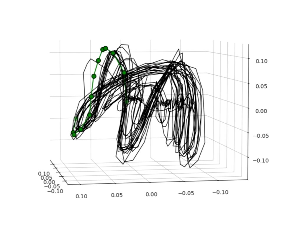Fig. Applause “Embedded segment from “Applause” by Lady Gaga. Green circles can be ignored; they are only used to synchronize audio in the corresponding video.

I embedded a sample of songs from diverse genres and rhythmic patterns. I synchronized them with their audio in Sony Movie Studio 16 Platinum. Watching and listening carefully is the best way to get a sense of why the embeddings look the way they do!

My method very often highlights the cyclic nature of the rhythm in these songs—making the embeddings almost too predictable at times. Many songs had an annular/”bird’s nest” structure, often with multiple lobes. This causes them to resemble strange attractors. However, in a system like the Lorenz equations, with an actual strange attractor, the solution curve will oscillate seemingly randomly between the two lobes. For music this does not happen; the curve traverses the lobes in a specific, repeating order. To borrow from dynamical systems theory, this makes the embedding more like a noisy limit cycle.

It’s important to note that, in the case of embedding music, the embedding space is technically not a proper “phase space” in the dynamical systems sense. For example, there’s no obvious analogy for having two different initial conditions in this space. It is, however, much like a phase space, and that is why cyclic patterns in the music are faithfully represented as loops.

I began to seek out songs that do not have such obvious cycles. For these the embedding is more complex and lacks a repeating orbit (See e.g. “Concerto…” - Vivaldi or “I love the woman” - Freddie King in video). It is still possible to understand their shape by listening.

Effect of conditioning on prediction

Recall that I conditioned the encoder by adding \(L_{forecast}\) to the loss function. This encourages the embedded points, produced by the encoder, to be useful for predicting the next time-step. This conditioning smoothed the embedding significantly for all songs sampled. However, it seemed to come at the cost of reducing spatial resolution of the lobes. Lobes of the embedding that were once separated tended to blend together when conditioning was applied. The impact on forecasting accuracy will be measured in the last section.

In the figure below is the embedding of a clip from “No Place to Go” by Eilen Jewell. (Right) comes from a pure convolutional autoencoder and (left) comes from placing the additional forecasting condition on the encoder.

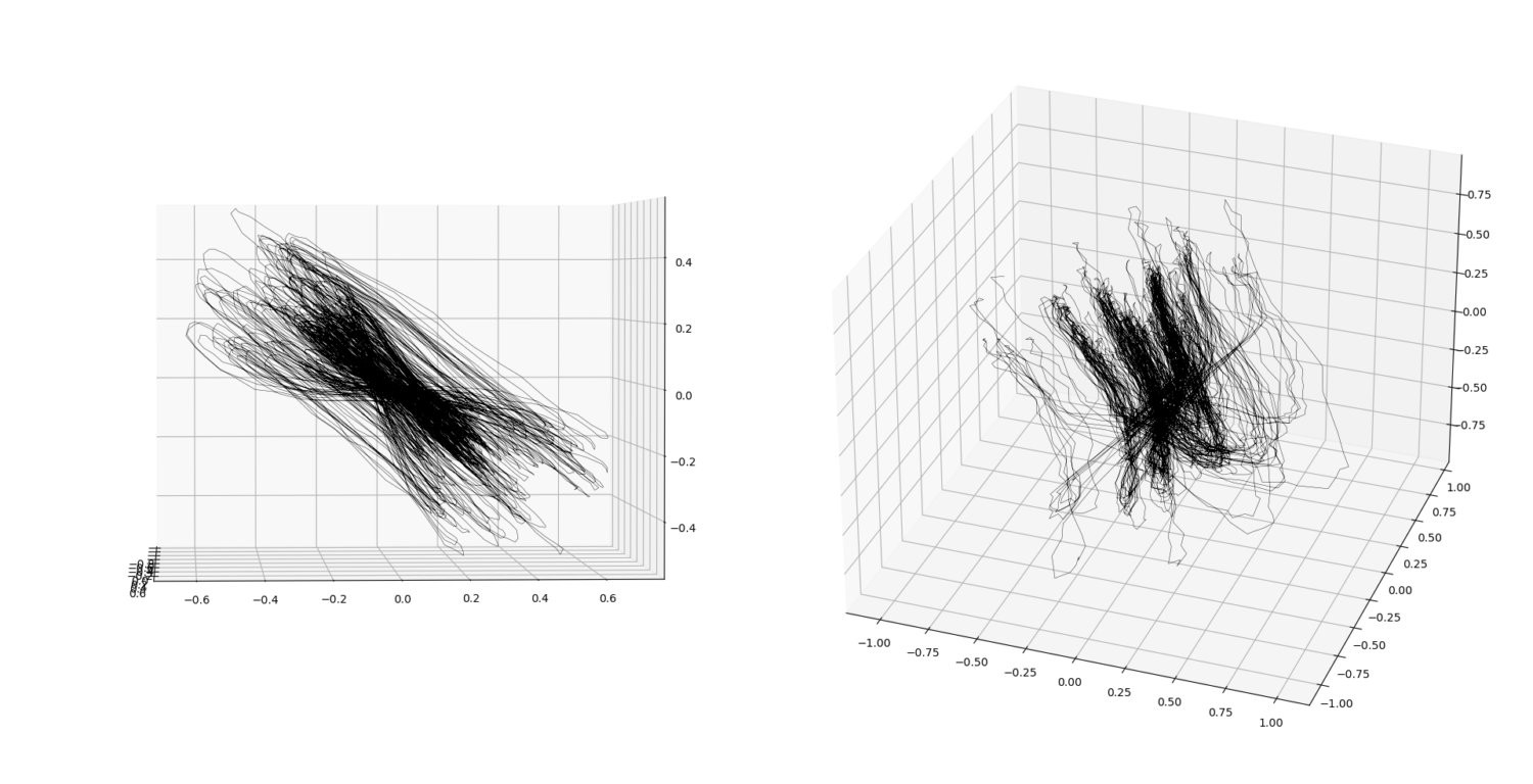
Fig. NPTG-R-RF Embeddings of “No Place to Go” by Eilen Jewell using a 0.5s window. (left) Using model trained with both losses \(L_{forecast}\) and \(L_{recon}\) on. I.e. encoder network was conditioned on forecasting. (right) Using model trained with only \(L_{recon}\) on. I.e. pure autoencoder.

Effect of window size

I experimented with two windows that were a factor 4x apart in width: 2s and 0.5s. Their embeddings differ dramatically. A 2s window (meaning 2s of audio is compressed to a single point) produced much smoother trajectories and captured longer time scale musical transitions. An embedding made with 0.5s window is much more expressive, capturing shorter time scale patterns, as one would expect. Below are the 2s (left) and 0.5s (right) embeddings of “Concerto for violin No. 4 in F Minor, Op. 8, RV 297 Winter I. Allegro non molto” by Antoni Vivaldi.

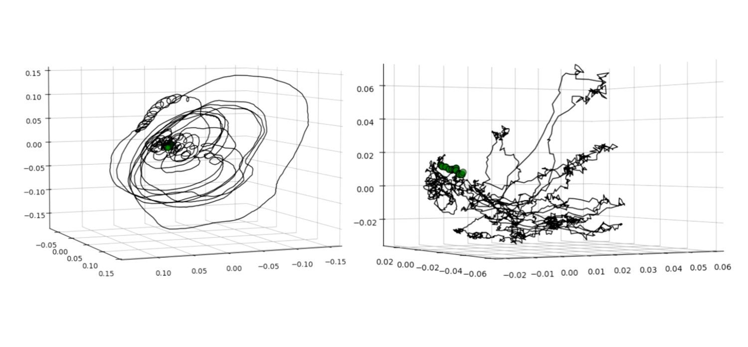Fig. Vivaldi-half-two “Concerto for violin No. 4 in F Minor, Op. 8, RV 297 Winter I. Allegro non molto” by Antoni Vivaldi. Sliding window length: 2s (left) and 0.5s (right).

Divergence of forecasted trajectory

Below are two example forecasts using the KNN-based interpolation method. Fig. NPTG-forecast 200 step forecast from random initial condition in “No Place to Go” by Eilen Jewell. This embedding came from the conditioned autoencoder with 0.5s window (the same data as Fig. NPTG-R-RF (left))

Fig. Vivaldi-forecast 200 step forecast from random initial condition in “Concerto for violin No. 4 in F Minor” by Antonio Vivaldi. This embedding came from the conditioned autoencoder with 2s window.

Examining the separation between true and forecasted trajectory \(\delta\) shows that prediction accuracy worsens quickly after only a few steps. This might be due to the very low amount of data used in the embedding (about 30s of audio). The red and black curves below compare the architectures with and without conditioning on forecasting. Conditioning on forecasting did lead to lower error, but only over the first few forecasting steps! I’ll give an possible explanation in the last section.

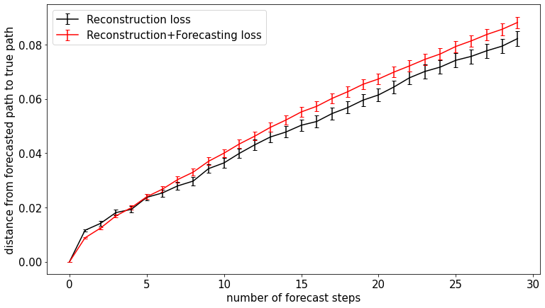Fig. NPTG-3D Mean \(\delta\) over forecasting steps in “No Place to Go” embedding. A 3D embedding space was used. Error bars indicate standard error.

Changing the embedding dimension from 3 to 12 exacerbated the difference between the two architectures. This suggests the source of error does not have to do with the limited capacity of 3-dimensional space. 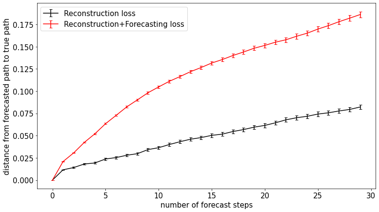Fig. NPTG-12D Mean \(\delta\) over forecasting steps in “No Place to Go” embedding. A 12D embedding space was used. Error bars indicate standard error.

The pattern is similar in the Vivaldi embedding. I did not run this analysis with any other songs. 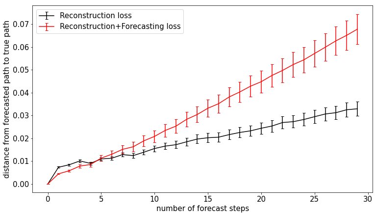Fig. Vivaldi-3D Mean \(\delta\) over forecasting steps in “Concerto for violin No. 4 in F Minor” embedding. A 3D embedding space was used. Error bars indicate standard error.

Conclusion | Why did forecasting accuracy get worse?

The forecasting error was lower in the conditioned embedding, but only over a very short time scale. This makes sense because the conditioned embedding was explicitly optimized to yield lower predictive error. Crucially, however, only the error over one time-step was considered. Specifically, the loss function’s \(L_{forecast} = 1 - CosineSimilarity(v_t, \hat{v_t})\) only compares the true \(v\) and predicted \(v\) at the current time-step.

It is possible that imposing this local constraint effectively distorted the global structure of the unconditioned embedding (produced by the pure autoencoder). And this lead to increased error in the long term.

The success of this project was in forming a novel representation of audio and music that matched reasonably well with our expectations. These type of embeddings could be used for downstream tasks such as rhythmic analysis or clustering songs by their rhythmic structure. This is a useful attribute that could be leveraged by music recommendation systems and other applications.

Thanks for reading!